There’s a lot of talk out there about using large language models to help testers write tests, such as coming up with scenarios. There’s also talk out there about AI based tools actually doing the testing. Writing tests and executing tests are both a form of performing testing. So let’s talk about what this means in a human and an AI context.

My focus here is going to be on reinforcement learning. I truly believe that any AI tool that will actually help humans with testing must be based on this broad style of algorithms.

Reinforcement learning, which is inspired by the way humans learn through interaction with some environment, is, I would argue, the most relevant concept in the context of AI testing tools. If you want AI to perform testing tasks similarly to humans, it should not only be capable of creating test scenarios but also executing them effectively.

Here’s the foundational question we’re really asking: can we give an AI a possibly ambiguous, certainly open-ended, relatively complex goal that requires interpretation, judgment, creativity, decision-making and action-taking across multiple abstraction levels, over an extended period of time? That’s the question to be asking because that’s what testing is all about.

Part of what human testers have to do is adapt their testing strategies over time and that adaptation comes about through investigation.

Read “investigation” as trial-and-error based exploration. That’s pretty much the entire basis of reinforced learning. That investigation may, but does not have to, become scripted exploitation.

Here I’m purposely drawing a distinction between the idea of tests as artifacts and testing as disciplined activity. Doing testing is what allows you to create tests. Testing is more about exploration while tests are more about exploitation.

Testing involves exploring and understanding an application’s behavior while creating tests can be seen as the exploitation of that knowledge to design specific test cases. As you’ll see, AI research is also focused on the distinction between exploration and exploitation.

I’ll note that you can also test more than just the application’s behavior. You can utilize testing to put pressure on design that will help form the specifications that say what the behavior should be. However, in this post, I’m going to focus on the idea of executing tests against some sort of application because that’s what the industry is most interested in right now.

Now if what I’m saying is true, and given the interest in AI overall, then testers should understand the basis of reinforcement learning. And this is actually really easy to do! But testers also should be able to explain why this model has relevance to those who are not testers. This blog post is my experiment to see if I can cater to both audiences.

I’m going to use a very minimal Python example in this post. It will require no specialized environment nor will it require any external libraries. If you have a basic Python implementation on your machine, you can play along. If you don’t want to type in the example, fear not! I’ll show the output and describe what’s happening.

The Basis of Reinforcement

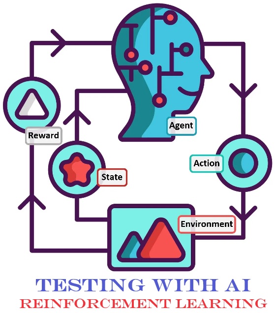
In the realm of reinforcement learning (hereafter, RL), we encounter two key players: the agent and the environment. Think of the agent as the decision-maker and the environment as the stage on which those decisions are enacted. Connecting these central components are three vital signals or messages: the state, reward, and action. You’ll often see this diagrammed out like this:

The state signal serves as a snapshot of the current state of the environment. It’s like a real-time photograph capturing where the agent finds itself in its surroundings. Imagine it as the current position of a robot in a room, for instance. Or, say, the current configuration of a chess board.

Rewards are the ‘good’ or ‘bad’ feedback the agent receives. The environment can provide these rewards as external feedback, but sometimes the agent generates them internally as well. For now it’s enough to understand that rewards are the guiding beacons that help the agent learn and adjust its behavior. Rewards are like the “carrots” and “sticks” that guide the agent.

Thus note that the term “reward”, while normally applied only to good outcomes, is used to indicate both good and less good. Think of it as a value that can be positive or negative.

Lastly, we have the action signal. This is the decision the agent makes at each time step within the environment. Picture it as the move a chess player selects during a game or the movement a robot chooses to take to cross a room.

Fundamentally, what you get is this:

The agent encounters the environment in some state (S). They take an action (a). Some reward (r) occurs and the environment is now in a new state (s').

These components are intertwined in a delicate little dance of exploration and exploitation, where the agent learns to make decisions based on the state and the anticipation of rewards, aiming to maximize its performance over time. The concept of exploration (trying out new actions to learn) and exploitation (choosing actions based on what the agent knows works well) is a fundamental aspect of RL.

It’s also a fundamental act of testing. This is exactly what humans do when they engage in the discipline of testing something.

So you might have a scenario like a robot (agent) navigating a room (environment), where the state is its current position, the reward is a score for the task it’s performing, and the action is the movement it chooses to take. Getting further from the other side of the room would be a negative reward while getting closer to the other side of the room would be a positive reward.

You could also apply this to a chess game where the player (agent) is navigating a chess board (environment), where the state is the position of all the pieces at a given time, the reward is a score for whatever movement is being considered, and the action is the actual movement being chosen. Making moves that increase the likelihood of checkmating the other player would be a positive reward while making moves that make yourself vulnerable to being checkmated would be a negative reward.

Think about what this positive/negative reward might be in the context of a tester who is testing an application. Getting closer to or further from the bug maybe? Ah, but how would the tester actually know that? Consider that same question in relation to: how does a chess player know they are getting further or closer to checkmaking the opponent? It all has to do with what’s observable and understanding how the environment state changes in response to actions.

The Fundamentals of Reinforcement

In the world of reinforcement learning, an RL agent is like a skilled player navigating its way through a game. To play this game, the agent is equipped with four essential tools: a policy, reward function, value function, and, optionally, a model.

• Think of the policy as the game plan, the strategy that the agent follows. It’s like a playbook for a sports team, guiding every move the agent makes. Or think of it like a chess player that knows all the standard opening move sets in a game of chess.
• The reward function is like a scoreboard. It keeps track of how well the agent is doing and provides feedback. Rewards can come from the outside world or be generated internally, just like scoring points in a game (external) and also a desire to score as many points as possible (internal).
• The value function acts like a player’s assessment of their progress. It’s crucial for making long-term decisions. Imagine it as a player deciding if they’re winning or losing in the grand scheme of the game.
• The model represents the game world, akin to having a detailed map. In simple games like tic-tac-toe, it’s like knowing every possible state of the board. But in complex games like chess, it’s more like having a general idea of the game board because there are too many possible positions to know them all.

Consider again my previous statement about how this relates to testing and the idea of what is observable. This ties into what we can model. Models can be definite and specific. They can also be heuristic.

So a way to bring all this together is to say that the policy is the decision-making strategy, the reward function guides learning, the value function assesses the long-term desirability of particular states, and the model represents the environment where state changes happen that allow for planning and learning.

Let’s Get Markovian

In the world of RL, the agent’s key to learning is understanding its surroundings, which are captured in the state signal. This state represents a snapshot of the environment, but it’s like looking at one piece of a puzzle. To make informed decisions, the agent needs more than just the current state.

That takes us to the idea of the Markov state. This is a special kind of state that has a bit of a superpower — it can predict the future! Well, sort of. Imagine it as a crystal ball that gives you a glimpse of what’s to come. Or, at least, what’s likely to come. In RL, we want to be able to predict what will happen next based on the current state.

When an RL problem fulfills this “crystal ball” condition for all its states, we say it has the Markov property. This means the agent can make decisions, predict future values, and navigate its way through the environment confidently.

When the Markov property is consistent across all the states in a learning task and that task is a finite problem, we call it a finite Markov Decision Process, or MDP. MDPs are like neatly defined puzzles, where the agent can piece together the future and make smart choices based on the current state.

“Markov,” by the way, is named after the Russian mathematician Andrey Markov, who made a lot of contributions to the field of probability and stochastic processes. He introduced the concept of Markov chains, which are mathematical models used to describe systems or processes where the future state depends only on the current state and not on the entire history of the system.

Solving an MDP

Okay, so what we end up with is a Markov Decision Process (MDP) concept.

It’s a model for how the state of a system evolves as different actions are applied to the system. The above visual shows a way this is often represented. What you see there is a “gridworld navigation task” where the robot not only has to find its way to the goal location (the green house) but also has to avoid trap locations (red signs).

So think about the “gridworld” as an application being tested. Or perhaps just one feature in an application under test. But, in that case, the red signs are the bugs. The green house is the outcome of the feature providing value. Keep playing this idea in your head as you go on through this post. Are humans and AI “solving” for the same thing?

So the main takeaway here is that an MDP is something to be solved. Solving a full MDP and, hence, the full RL problem around it, first requires us to understand values and how we calculate the value of a state. We do this with a value function.

I’ll reinforce my above statement yet one more time. As we go on here, I’m going to ask you to abstract things a bit. As I talk about these concepts, think about how they apply in the context of a human tester taking actions with an application. Because if we’re asking AI to do something similar, and determine value or lack thereof, it’s critical to understand how these concepts translate between AI and human.

Determining Value

Here’s the basic equation you can consider for now:

Here a is the action taken, r is the reward we get from taking the action, the α refers to the concept of a “learning rate.” Thus this function — V(a) — refers to the value for a given action.

I’ll talk about the learning rate in a bit but for now let’s explore this with code. Specifically, let’s create a very small program that effectively demonstrates how an agent can update its estimated values for different actions over multiple episodes using the learning rate and the received rewards. And I should note that an “episode” in the context of RL typically refers to a single run or iteration of a learning process. It represents a sequence of actions and interactions between an agent and its environment. An episode is thus a self-contained learning session.

Think of an “episode” as perhaps running one test against a feature. Or as a series of tests against a feature.

If you want to play along, create a Python script called value-learner.py. In that script, put the following:

You might wonder what “arms” refers to here. This terminology has to do with what this example represents, which is often called a “multi-arm bandit” scenario. I’ll come back to the meaning of this but for now just understand that a multi-arm bandit scenario is like a casino game where you’re faced with multiple slot machines (arms), each with its own unknown payout rate (reward).

The challenge — and thus the problem to solve — is to figure out which machine has the highest payout without knowing any of the true payout values. To do this, you have to decide how much to “pull” each arm (explore) to gather information about their payouts and then allocate more pulls to the machine with the highest expected return (exploit) as you learn.

You might get something like this when you run this script:

[0.814697981114816, 0.3587852317595, 0.1629395962229632, 0.26085155000000004, 0.5270540072456584, 0.08784233454094308, -0.30628975550000004]

This output represents the estimated values for different actions after the agent has gone through the learning process. But what does this actually mean? Let’s break it down.

• Each number in the output corresponds to the estimated value of taking a specific action with a specific arm. These values are the agent’s best guess of how valuable each action is in the given environment.
• In the context of this script, these values help the agent decide which action to take. A higher estimated value indicates that the agent believes that action is likely to yield better rewards in the long run.
• Over the course of 100 episodes, the agent has learned and updated its estimated values for each action. It started with all values set to 0 and adjusted them based on the rewards it received during its interactions with the environment, meaning by “pulling each arm.”
• The action with the highest estimated value is considered the optimal action. In this case, the action with the highest estimated value is the one the agent believes will, on average, yield the most significant reward.

What you really want in any learning scenario is something called convergence. In an ideal scenario, the estimated values should converge towards the true values of each action, providing the agent with an increasingly accurate assessment of which actions are most profitable. So, in essence, these values are the agent’s way of learning and making informed decisions by estimating the potential return associated with different actions. They guide the agent in selecting actions that are likely to maximize its rewards over time.

So as a tester maximizing my rewards over time, I want to be making assessments about possible risks around how an application behaves and thus how, or whether, it provides valuable outcomes to users. What this means is that one of my rewards are finding value threateners, which we might label “bugs” for now.

Now, I don’t know about you, but when I first came across examples similar to this it all seemed … well, to be honest, entirely useless. After all, the rewards are listed as part of the code. We know that that first reward is 1.0 and so that’s effectively “best.” Wouldn’t the “agent” know that as well?

And, yeah, that’s a valid point. But this reflects a common misunderstanding about the example. In this simple example, it’s certainly correct that the rewards are known and the highest reward is 1.0. However, the purpose of this code is to illustrate the fundamental concept of how an agent learns and updates its action values over time. So here’s how I learned to deal with my skepticism on how useful this really was as a starting point for learning.

1. The example is designed to provide a simplified illustration of the RL learning process. In real-world RL applications, the agent often doesn’t know the true rewards in advance and thus it must learn them through interactions with the environment.
2. Imagine a scenario where the agent doesn’t initially know the rewards for each action. It explores and takes actions, gradually learning which actions yield higher rewards and updating its estimates accordingly. The goal is for the agent to make good decisions in situations where the outcomes are uncertain.
3. So while this specific example might not fully demonstrate the challenges of RL, the same principles apply to much more complex scenarios where the reward landscape is unknown and constantly changing. The agent’s ability to learn from interactions becomes crucial in such situations.

So, above, when I talk about allowing the “agent to make good decisions in situations where the outcomes are uncertain”, consider that statement in relation to a tester making good decisions and where to apply different techniques of testing given that we may not know where bugs are lurking or what type of bugs exist and where they don’t have an infinite amount of time to find them.

What you should take from what I just showed you here is that this very basic example is a stepping stone to understanding more advanced RL algorithms. Some of those go by names like Q-Learning and Deep Q-Networks, the former of which I’ll cover in this post. These more advanced methods apply the exact same principles but in much more complex environments where the true reward function isn’t known.

Linking the AI and the Human

These stepping stones, simple as I realize they are, show us how we have to think about an AI that’s truly doing testing in any way that we could call similar to how a disciplined human would do so. So keep in mind that what we have right now is this:

Here you basically have a known reward. But what we really want is something like this:

What I hope you take from this is that this extremely simple code demonstrates the core concept of RL — how an agent learns from experiences to make better decisions. While the rewards are known here for simplicity, the same principles apply to situations where those rewards are uncertain and must be discovered through exploration and learning. And I’m reinforcing this point yet again because this is the situation testers find themselves in pretty much all the time.

Speaking of the “learning” part, I should call out that the learning rate of 0.1 that I used means that, in each iteration, the agent adjusts its value function by 10% (1/10th) of the difference between the received reward and the current value estimate for the chosen action. So what’s happening here is this:

• The agent takes an action, observes a reward, and computes the difference between the reward and its current value estimate for that action.
• The learning rate, in this case, 0.1, determines how much of this difference is used to update the value estimate. It’s like saying, “I’ll update my estimate by 10% of how different this reward is from what I expected.”

Over multiple episodes, and remember we’re doing one hundred of them here, this process of adjusting the value estimates with a learning rate helps the agent converge toward more accurate estimations of the values for each action, reflecting the long-term rewards those particular actions are likely to bring. This process of averaging out values across episodes is an essential aspect of reinforcement learning that allows the agent to make better decisions over time.

This is exactly what humans do when exploring and learning as well. This isn’t surprising since RL techniques were developed and adapted based on how humans seem to operate.

And speaking once again of “learning,” I most definitely need to point out that this agent isn’t really learning. Look at the code again and see what our agent is doing. It’s just randomly picking an arm each episode. The agent isn’t using its acquired knowledge from the value function to determine its next best choice. What this means is that the agent really has no decision mechanism which is called a policy in RL.

Let’s Use a Policy

So let’s give our agent a policy. Here’s a modified version of the script, with the new or changed lines called out.

Here our agent becomes “greedy.” The greedy() function is essentially the agent’s policy, which always selects the action with the highest estimated value. This policy guides the actions of the agent. The output will likely be something like this:

[0.9999734386011123, 0.0, 0.0, 0.0, 0.0, 0.0, 0.0]

Hmm. That seems very different than what we got before. And that probably makes sense since I’m saying that having a policy impacts the agent’s ability to make better choices. But are we seeing “better choices” here? Well, what that output shows us is that the agent calculated the maximum reward arm correctly, but likely didn’t determine the correct values for the other arms. The reason for this is that as soon as the agent found the most valuable arm, it kept pulling that arm. So essentially the agent finds the best path and sticks with it. Let’s make sure we understand what’s happening here and, as we do, think about what this might correlate to with someone who is testing an application.

• The output, with one action having a significantly higher value than the others, indicates that the agent correctly identified the arm with the maximum expected reward.
• The agent’s strategy, in this case, is to “exploit” the best arm and stick with it because it has learned that this action provides the highest rewards.

Maybe we have a tester who is relying solely on a scripted test case to test a feature because, at one point, that test case exposed a bug. And this tester counts the reward as the running of this test case and finding no regression. Maybe another tester counts the reward as the running of this test case and finding a regression. Notice how the reward function differs quite a bit here.

While this greedy approach might work in a simple, single-step or stationary environment, it won’t be effective in scenarios that involve multiple steps or changing conditions. In such situations, exploration (trying out other arms to discover potential better options) is essential for long-term success. I’m going to come back to this idea of stationary environments in a bit and contrast that with non-stationary environments.

Let’s Get Optimistic

When our agent consistently chooses the best-known option, it clearly restricts its ability to explore and learn in-depth about the environment. This not only limits the agent’s understanding of a single state but also hinders its capacity to navigate complex environments with multiple interconnected states. So what we need here is a more balanced policy, one that encourages both exploration and exploitation.

In essence, we want to find a policy that allows the agent to venture into the unknown while also capitalizing on its existing knowledge. This balanced approach is crucial for maximizing the agent’s learning potential and adapting to environments with varying challenges and opportunities. What this is capturing is the core problem of an agent that always makes the “best” choice without exploration. I want to emphasize to you the limitations of such a strategy in learning complex environments.

Again, think about how that applies in testing. We would risk missing subtle bugs at the expense of finding what we might call “surface” or “shallow” bugs. It’s not that the surface bugs are unimportant necessarily but, rather, that too much a focus on them might forestall finding more subtle or “deep” bugs. The converse is also true: we could spend so much time doing very deep that we miss whole swathes of bugs on the surface.

Let’s see if we can find a slightly better policy. In the code we created, change the episodes and value variables as such:

Just making these changes effectively introduces a technique known as “optimistic initialization.” This can be highly effective in motivating the agent to explore all available actions. Let’s talk about what’s better about this approach.

• By setting the initial values higher than the possible rewards (5.0 is much higher than 1.0), you effectively force the agent to explore all actions, ensuring it doesn’t prematurely converge to a suboptimal strategy.
• This allows the agent to learn quickly in the early episodes, where it tries each action at least once. This can provide a more comprehensive understanding of the environment.
• Once the agent has tried all actions, it can transition to a more balanced exploration and exploitation strategy, using its learned values to make informed choices.

This approach is flexible and adaptable to different types of environments, making it a useful technique in the RL toolkit. However, it’s important to keep in mind that the effectiveness of optimistic initialization depends heavily on the specific characteristics of the environment and the learning algorithm used. For example, as I’m sure you can imagine, in some scenarios, this technique can lead to unnecessarily long exploration phases. So it’s essential to balance this technique with other exploration strategies when needed.

I should note here that my game Test Quest was designed to look for how testers utilized an exploration versus exploitation dynamic in their testing, essentially seeing what balance they ended up with.

What’s interesting here, I think, is that the output will be something like this:

[1.0000000000000009, 0.9923854510918054, 0.9204542494255955, 0.9923854510918054, 0.9899692772647101, 0.9171819032836618, 0.8980262055809499]

This can be subtle but what I want to call out is that the calculated values are now more relative than they were in previous outputs. That is, the value of 1.0 clearly indicates the best course of action here — the arm with a reward of 1.0 — but the other values are less indicative of the actual reward and are more relative to that 1.0 that was calculated.

So what this means is that the output values reflect the relative estimates of different actions in the environment, considering the optimistic initialization. While the value of 1.0 for one action clearly indicates its high reward, the other values are more relative to this maximum. They represent the agent’s learned estimates of how good the other actions are compared to the best-known option, which has been set to 1.0.

In essence, these values provide a sense of the agent’s assessment of the actions’ relative desirability, emphasizing the importance of their order rather than their absolute magnitude. This approach allows the agent to make choices based on the order of action values, enhancing its adaptability in dynamic environments.

This is critical because the idea of order gets into the notion of causality. And testing is all about causality. That means an AI acting as a disciplined tester must have some notion of causality.

I can’t stress enough how easy it is to show these examples in relatively simple code. And this relatively simple code is, I assure you, the basis behind the more complicated algorithms that are out there. And I can further assure you that these concepts are exactly what humans are doing, albeit with more nuance, when engaging in situations where they have to make decisions under conditions of varying uncertainty.

We Still Need Balance

Okay, so our greedy approach effectively only had the agent exploring one path. Our optimistic approach had the agent exploring all paths. What we want to do is find a balance of exploration versus exploitation.

My example so far has been on the multi-arm bandit idea. Specifically, my focus has been on the stationary or non-contextual multi-armed bandit problem. This goes back to something I mentioned earlier. We can distinguish between stationary (non-contextual) and non-stationary (contextual) multi-armed bandit problems.

• In a stationary bandit problem, the rewards associated with each arm remain fixed over time. The agent’s goal is to learn the best arm to pull to maximize its cumulative reward. Typically, in each episode, the agent can pull one or more arms, with the aim of learning which arm yields the highest reward. This is the classic multi-armed bandit problem we’ve been working with here.
• In a non-stationary bandit problem, the rewards associated with arms can change over time. This can be due to various factors, such as external influences or changes in the environment. In this scenario, the agent’s task is to adapt to changing reward distributions. Often, the agent must decide which arm to pull in each episode based on the current context, making it a more dynamic problem.

So in my examples so far, I’ve primarily focused on the stationary multi-armed bandit problem, where the rewards are fixed and the agent learns to choose the best arm over episodes. However, what I really want you to understand is that the concepts I’ve covered are foundational and can be extended to non-stationary or contextual bandit problems where the agent adapts to changing reward distributions or contextual information. And I want you to understand that because that’s how you see to scale these examples to closer to what happens when humans used reinforced learning.

So, with that said, I’ll now follow the natural progression in reinforcement learning.

Getting Into Quality Learning

Let’s move from our simple multi-armed bandit scenario to a more complex environment with states and actions and, in this new scenario, the goal will be to determine the quality of actions within different states. Q-learning is an excellent approach for achieving this. Q-learning, which relies on something called the Bellman equation, is well-suited for problems where an agent interacts with an environment, observes states, takes actions, and receives rewards. It allows the agent to learn the quality (value) of actions in different states, facilitating more complex decision-making in dynamic environments.

If you follow me on this progression, this aligns with the broader concepts of reinforcement learning and sets the stage for exploring more advanced RL techniques and applications and, I might add, gets you closer to understanding why this kind of AI would be a necessary start towards acting like a human who is performing disciplined testing.

So, first, here’s the equation:

I actually would prefer to show you this a bit more programmatically, so let’s go with this:

Q(s, a) = Q(s, a) + α × (r + γ × max(Q(s', a')) - Q(s, a))

Here s is the current state. And s' is the next state. That means a would be the current action and a' would be the next action. The α is, as before, our learning rate. The γ refers to a reward discount. Don’t worry terribly much about understanding all of this right now. What I want to do here is link the Q-learning equation to the earlier action-value equation. I want to highlight the evolution of the concept from action-values to Q-values and how this allows the agent to plan and make decisions in a more comprehensive manner across multiple states.

I’m doing this because I’m hoping this helps you understand the transition from simple reinforcement learning scenarios to more complex ones where the agent considers not just the immediate reward but also the potential future rewards and optimal actions.

So here I would recommend just creating a new script, perhaps called q-learner.py. In that script, put the following:

Notice that I’m initializing the arms variable to 7 and then a new bandits variable to 7 as well. Also notice that now the reward list is no longer filled in. So the agent has no idea what the rewards are. I print the Q value twice and the calculated rewards as well. So in the output you might see this:

[[0.7898266795171887, -0.011730610089010662, 0.8414414492250899, 0.9807552478948365, -0.8956136252271807, -0.5568710465147464, -0.15173040656154213], [-0.8957688532075283, -0.8361968042041568, 0.8485551116501464, 0.6066278627373693, 0.2734167444969098, 0.9014167273471341, 0.771607417868954], [0.4407336935349584, -0.3820414296459196, -0.0010744279285967995, 0.5811433936874997, 0.5265024995281278, -0.3552339070437125, 0.6042275102762893], [0.00033501475131658687, 0.6902221768601182, 0.9863497597455471, 0.2631667862187508, 0.29825403454940913, -0.3753843898745146, 0.9125390142008374], [0.8006983168370778, -0.8420501137243659, 0.8684385236637235, -0.9649608392815594, 0.722119140294706, -0.8468959050069393, -0.10066040209946747], [0.06154447543966812, 0.707857586969979, 0.9503497368741816, 0.19964021462480375, 0.7718287779642039, 0.6491897743430008, -0.4047557916603788], [0.026018153364450347, 0.4212651392304294, -0.3725361949254178, 0.08113375650142363, -0.1495678961261171, 0.7059735040945061, -0.646559644307694]]

[[10.0, 10.0, 10.0, 10.0, 10.0, 10.0, 10.0], [10.0, 10.0, 10.0, 10.0, 10.0, 10.0, 10.0], [10.0, 10.0, 10.0, 10.0, 10.0, 10.0, 10.0], [10.0, 10.0, 10.0, 10.0, 10.0, 10.0, 10.0], [10.0, 10.0, 10.0, 10.0, 10.0, 10.0, 10.0], [10.0, 10.0, 10.0, 10.0, 10.0, 10.0, 10.0], [10.0, 10.0, 10.0, 10.0, 10.0, 10.0, 10.0]]

[[8.292369967579397, 7.184778562844144, 8.701247396712361, 8.450158514212639, 6.567007190712648, 6.441341171349627, 7.186474131242859], [6.622615612542188, 6.451828059824471, 8.716495610494256, 8.055563366904716, 7.856510202440893, 7.9138015537946895, 8.133826746472732], [7.949650776320552, 6.854895238164696, 7.946017272141868, 7.949242365939739, 7.9358627273260876, 6.654493154452374, 7.93103626282208], [7.478270863134069, 7.903361204520106, 8.81248881023933, 7.698903765898952, 7.756182016938856, 6.611265303769565, 8.196565780037425], [8.28945048507567, 6.502005090155618, 8.712381214443736, 6.627421525707325, 8.184097031525596, 6.153293115714473, 7.276665090757517], [7.4029702695832045, 8.057275677528803, 8.857183592718126, 7.720487877448282, 8.216395188594747, 7.643011874177986, 6.957193723595844], [7.521811431293392, 7.714591168532948, 7.549697221795842, 7.620226441940558, 7.286632249374551, 7.730825245717792, 6.638871565896043]]

The outputs are first the rewards and then, next, the Q-values that the agent has learned after multiple episodes.

Why all those 10.0 values? Remember that’s the optimistic one. This is just like how we used 5.0 in the previous example.

There are a few points I want to call out here.

1. The Q-values are not the same as the immediate rewards for each arm pull. Instead, they represent the agent’s learned assessment of the expected cumulative reward over time for each possible state-action combination.
2. The agent uses these Q-values to make decisions. It might explore initially by taking actions with uncertainty (higher variance in Q-values) and learn over time which actions in which states yield higher cumulative rewards.
3. As the agent learns, its strategy changes. It starts with a more exploratory approach, but as it accumulates knowledge (as indicated by higher Q-values), it becomes more exploitative, favoring actions with higher Q-values.

Again, I’ll ask you to reflect how this might play out with a human tester who is testing a particular feature in an application.

Do You See a Problem?

The problem with our current solution and using the full Q-learning equation here is that the equation assumes any state our agent is in affects future states. Except, remember in our example, the agent just goes randomly from bandit to bandit. This means using any previous state information wouldn’t really mean anything. So the agent moves randomly from bandit to bandit and, crucially, there’s no clear influence of one state on another. This makes the concept of discounted rewards less relevant in this specific scenario.

We can easily account for this by removing the concept of discounted rewards entirely. Specifically in my code I could change the learn() function like this:

Here I’m showing the commented out part of the statement that we previously had. What this change does is essentially remove the consideration of future states in the Q-value update.

There’s a caveat here. It’s important to note that the choice to include or exclude the discount factor should align with the nature of the problem you’re modeling. In more complex RL problems, where states do influence future states, the discount factor can be critical for making informed decisions and optimizing the agent’s behavior. In the simplified example we’re looking at, removing it makes sense.

Again, reflect on how this correlates with how humans test an application.

Discounting Rewards

I keep mentioning this idea of discounted future reward. But what does that actually mean?

Discounting future rewards is a way to give less importance to rewards that an agent may receive in the distant future compared to immediate rewards. It reflects the preference for immediate gains over long-term outcomes in decision-making. In our context here, I’m temporarily setting aside this consideration to better match the specific characteristics of the example, where the agent’s actions have limited influence on future states.

Make sure you understand why this isn’t needed in my code example. In my example, where the bandits (states) are not connected and the agent randomly transitions from one bandit (state) to another with no clear influence of one state on another, the concept of discounted rewards is less relevant.

Discounted rewards are typically used in environments where the sequence of actions in one state can significantly affect the outcomes in future states. Since there’s no such interdependence in my example, removing the discount factor is a reasonable choice to better align the algorithm with the characteristics of the problem I’m simulating.

Let’s Get Reductive!

And, taking all of what I just said into account, here’s something interesting. Well, to me anyway.

By omitting the discounted rewards component in my calculation, I’m actually simplifying the problem to a more straightforward value calculation problem! In other words, by omitting the discounted rewards part of the calculation, I’ve effectively just reverted to a value calculation problem.

I want to make sure you understand this. Specifically, I want you to see how the more complex Q-learning equation simplifies to the less complex value calculation equation when you remove discounts. Let’s go through this schematically. First, here’s our original Q-learning equation:

Q(s, a) = Q(s, a) + α × (r + γ × max(Q(s', a')) - Q(s, a))

Simplifying by removing discounts (setting γ to 0):

Q(s, a) = Q(s, a) + α × (r + 0 × max(Q(s', a')) - Q(s, a))

Simplifying further, clearly 0 × max(Q(s’, a’)) is 0:

Q(s, a) = Q(s, a) + α × (r - 0)

A further simplification (since r – 0 is r):

Q(s, a) = Q(s, a) + α × r

As a result, we end up with the value calculation equation:

V(a) = V(a) + α × (r - V(a))

This schematic representation shows how removing the discounts simplifies the Q-learning equation back to the more basic value calculation equation. I think this is a pretty clear way to illustrate the relationship between the two equations when discounts aren’t considered. But, wait. Are those equivalent? Consider we have these two equations:

Q(s, a) = Q(s, a) + α × r
V(a) = V(a) + α × (r - V(a))

They look almost the same. But the last part is clearly different. There’s an important distinction, for sure.

• In the Q-learning equation, you’re updating the Q-value directly with the received reward (r). This is common in Q-learning, where the agent is learning action-values.
• In the value calculation equation, you’re updating the estimated value (V) based on the difference between the received reward (r) and the agent’s current estimated value (V(a)). This is a typical representation in value iteration methods.

The key difference is that in Q-learning, you’re specifically learning different action-value pairs, while in the value calculation equation, you’re updating the value estimate based on the difference between the observed reward and the current value estimate for the same state-action pair. The “- V(a)” part represents the difference between what the agent expected (V(a)) and what it actually received (r), which is not present in the Q-learning equation.

So the end results may look somewhat similar, but the interpretation and purpose of these equations are different, and that “- V(a)” term in the value calculation equation represents the learning and adjustment of value estimates.

What I hope you can see here is the fundamental concept of how an agent learns to estimate the value of taking specific actions in different states without the additional complexity introduced by discounting future rewards. What you have here is, hopefully, an effective way to clarify for yourself the impact of the discount factor on a given problem.

Whew! Okay, bear with me here. We’re almost done. We’re actually at the crucial point but I needed all of the above to bring the crucial point home.

Let’s Be a Bandit

So let’s go back to talking about a multi-arm bandit here.

Ah, no, not that. Rather, this:

Let’s say you walk into a casino and you see three slot machines. Let’s also say that these are machines that are not guaranteed to have the same return. A hypothesis you have, in fact, is that one of those machines consistently has a higher rate of return than the others.

But how do you figure out which machine it is?

Think about how you might be testing a feature in an application and you’re pretty convinced one aspect of the feature has a bug. You have to figure out which part of the feature is not working. You have to figure out the right way to test it to prove that out.

By comparing the situation of choosing a slot machine in a casino to identifying a bug or issue in a feature of an application, we’re effectively illustrating the challenge of pinpointing the source of a problem among multiple possibilities. In both scenarios, there’s uncertainty about which option is the most favorable or which part of the system may have an issue.

Going back to the machine example, one strategy to find out which one, if any, is giving a higher rate of return is to try and figure out the return for each machine before spending the majority of your money. Certainly you could put the same amount of money into each machine and then compare the return, right?

And once you’ve finished doing that, you’ll have a good idea of which machine has the highest return. Then you can spend the rest of your money — assuming you have any left, that is — on that machine. But while you were testing, you put a fair amount of money into machines that have a lower return rate. You have maximized certainty but at the expense of maximizing revenue.

Just as in the casino, where you can choose to distribute your money among different slot machines or concentrate your spending on one, testing also involves the allocation of resources (in this case, time and effort) among various aspects or areas of a given feature.

This highlights the trade-off between maximizing certainty (finding a bug or issue with confidence) and maximizing coverage or the depth of testing. By focusing heavily on one aspect, you may become more certain about its status but potentially miss issues in other areas. Conversely, distributing your testing effort equally among different aspects may provide broader coverage but with less certainty about any particular one.

Interestingly, I think, this is also analogous to A/B testing.

In A/B testing, like in the multi-arm bandit scenario, you’re faced with the challenge of choosing between multiple options (A and B in this case) to determine which one performs better. Just as in the casino analogy, where you’re deciding which slot machine yields the highest return, in A/B testing, you’re trying to identify which version (A or B) leads to better outcomes, such as higher conversion rates or better user satisfaction.

The key similarity lies in the balance between exploration and exploitation.

Initially, you explore by assigning a portion of your audience to each variant (A and B) to collect data and determine their performance. This is akin to trying out different slot machines. As you gather data, you become more certain about which variant is more effective, and you can then exploit that knowledge by directing the majority of your audience toward the better-performing variant.

However, much like in the casino scenario or the focused testing scenario, during the exploration phase, you might lose some potential gains by diverting traffic to the less effective variant. It’s a trade-off between maximizing certainty about which option is superior and maximizing the overall outcome (revenue, conversion, satisfaction, etc).

Let’s go back to our machine example here.

We just talked about maximizing certainty at the expense of revenue. Flipping that around, there’s certainly a way to maximize revenue at the expense of certainty. Imagine you put a small amount of money in each machine and looked at the return. The machine(s) that returned the most, you place more money into the next round. Machines that return less, you put less money into.

Keep repeating and adjusting how much money you’re putting in each until you’re fairly certain which machine has the highest return. Or until you’re out of money, I guess. In this way you’ve maximized revenue at the expense of statistical certainty for each machine. You’ve avoided spending too much money on machines that don’t have good returns.

Just as in the scenario where you adapt your betting strategy based on previous returns from the slot machines, in testing, you can adjust your testing strategy based on the outcomes you observe during testing.

By allocating more resources to areas or aspects of the software that show issues or potential for improvement and scaling back in areas where you’re not finding problems, you are essentially applying an exploration-exploitation strategy. This way, you aim to maximize the effectiveness of your testing by focusing resources on areas that are more likely to yield valuable information.

The Fundamental Meaning

What I’ve tried to show you here is that the idea of an explore-exploit dynamic is at the heart of testing.

The explore-exploit dynamic is a fundamental concept not only in testing but also in various domains, including science and experimentation. In science, researchers often need to strike a balance between exploring new, uncharted territories (exploration) and exploiting what they already know to make meaningful discoveries and advancements.

This dynamic is essential for optimizing the allocation of resources — whether that’s time, effort, or funding — to maximize the chances of achieving the desired outcomes. In the context of testing, experimentation, or scientific research, finding the right balance between exploring new possibilities and exploiting existing knowledge is key to making progress and achieving meaningful results.

What I’m describing here is a universal concept that applies to problem-solving and decision-making in many areas of human endeavor, particularly where those endeavors have more or less uncertainty associated with them.

This reinforces a lot of ideas I’ve talked about in the past on this blog, which is that testing is predicated upon the scientific method. Testing is a form of experimentation. In fact, testing is experimentation. The feedback from our experiments is how we come to understand how well or how poorly something behaves or operates in a given context.

The quicker we achieve this feedback, and the more we scope our experiments to be small, the more chance we have of finding our mistakes as quickly as we make them, which shortens our cost-of-mistake curve. A short cost-of-mistake curve is a great way to balance exploration and exploitation.

Testing is thus not just about finding bugs but also about gaining insights and knowledge about whatever it is we’re testing and forming assessments based on perceived risks. We confirm, we falsify, and we implausify.

This is an insider view of testing. And it’s the view that skilled practitioners must show to outsiders to testing.

But it’s also one that we can further situate within the context of those who want to talk about what an “AI doing testing” would look like. Remember the question I asked at the beginning: can we give an AI a possibly ambiguous, certainly open-ended, relatively complex goal that requires interpretation, judgment, creativity, decision-making and action-taking across multiple abstraction levels, over an extended period of time?

This post was the start of showing you how to explore that question.