This post continues on from discussing the theory around path testing. Now I want to put some of that theory into practice. While this is geared toward testing, it by necessity jumps into the programmatic side of things. I think this is an important view for testers to have.

From the last post, we know a few things:

• Program graphs are a graphical representation of a program’s source code.
• A path through source code can be linearly independent.
• A path is linearly independent from other paths if it includes a path that hasn’t been covered before.
• A test strategy is to find the total number of linearly independent paths and cover them with data conditions.
• Those data conditions will exercise boundary conditions and logic paths.

This takes us straight into the technique of path coverage.

Path Coverage

Path coverage refers to designing test cases such that all linearly independent paths in the program are executed at least once. A linearly independent path can be defined in terms of what’s called a control flow graph of an application.

Great. So what exactly is a control flow graph?

This is simply a visual way to describes the sequence in which the different statements of an application get executed. In other words and perhaps not too surprisingly given the name, a control flow graph describes how the control flows through the application. The control flow graph for any program (no matter how small or large) can be easily drawn if you know how to represent various language statements or structures. To show that this is not all some academic theory, here are some examples of control flow graphs for very common constructs that you’ll find in most programming languages:

IF construct

UNTIL construct

WHILE construct

From a developer perspective, in order to draw the control flow graph, all the statements of a particular part of the application must be numbered. The different numbered statements serve as the nodes of the control flow graph. An edge from one node to another node exists if the execution of the statement representing the first node can result in the transfer of control to the other node. (Check out my previous post where I showed graphical representations of nodes and edges.) I’ll give some actual examples of this in a little bit.

Combined with what I just said and simply by looking at the above (admittedly sparse) examples of graphs, you can see that there are a few ways to consider coverage from a testing standpoint.

• Node Coverage: Achieved when the paths identified have a test that goes to every node in the graph.
• Link Coverage: Achieved when the paths identified have a test that goes along every link, or line, in the graph. In many cases, node coverage will take care of this.
• Loop Coverage: Achieved when the numerous paths identified have tests that explores the interaction between sub-paths within a loop.

Let’s consider this with a specific example. Here’s a control flow graph:

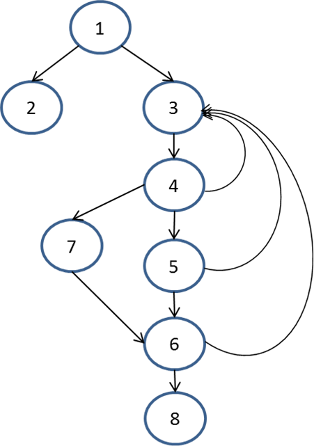
Going with the above testing coverage ideas, this table lists the test paths you could consider through the program flow.

Node Coverage	Link Coverage	Loop Coverage
1 2	1 3 4 3 4 5 3 4 5 6 8	1 3 |4 3| 5 7 8
1 3 4 7 6 8		1 3 |4 3| 7 6 8
1 3 4 5 6 8		1 3 4 |5 3| 4 5 6 8
		1 3 4 |5 3| 7 6 8
		1 3 4 5 |6 3| 4 5 6 8
		1 3 4 5 |6 3| 4 7 6 8
		1 3 4 7 |6 3| 4 5 6 8

In the Loop Coverage column, I used pipe characters to show where a specific loop was being entered. As an exercise for you to think about, consider that you could replace the third node test with the link test. That would mean you only needed two node coverage paths.

Realistically, it’s important to note that just using this graph, you really don’t know the data conditions that would differentiate the 4 –> 3 link from the 4 –> 5 link or the 4 –> 7 link. Those may require more tests based on the specific conditions. This is an important caveat and it’s one that plaques unit testers everywhere: just because you have coverage, doesn’t mean you have effective coverage.

Graphing the Coverage

So now let’s talk a bit about different measures of coverage. This will help you understand how path coverage is built up from lower-level ideas.

Statement Coverage

One of the lowest level types of coverage you can get is coverage at the statement level. Statement coverage is a metric that tells you whether the flow of control reached every executable statement of source code at least once. Thus from a testing perspective, the goal is to identify a set of test cases that are sufficient to exercise all statements at least one time. The idea is that you number each executable statement. Here’s an example of some simple Java logic:

    public class compute {
      public static void main(String[] args) {
(1)     float x = Float.valueOf(args[0]);
        float y = Float.valueOf(args[1]);
(2)     if (x != 0)
(3)       y += 10;
(4)     y = y / x;
(5)     System.out.println(x + " " + y);
      }
    }

Notice here that only executable statements are numbered. Also notice that you can group some statements together as I did with the declarations for the x and y variables. Here’s what a control flow graph of this situation would look like:

You can see what path is taken when the variable x is equal to 0 and when the variable x is not equal to 0. This certainly seems like you have adequate coverage to catch any bugs. Yet there’s a problem. Even in a case of a program without iterations — like this one — the execution of every statement does not guarantee that all possible paths are exercised. Consider the following test set:

• x = 1, y = 2
• x = 2, y = 1

These tests cover all of the statements. Yet notice that by pure statement level coverage, the potential error of division by 0 is not identified (statement 4).

What this shows you is that you need to look beyond just statements. The fundamental assumption of code coverage testing is that to expose bugs, you should exercise as many paths through your code as possible. The more paths you exercise, the more likely your testing is to expose bugs. So let’s consider two points here:

• A path is a sequence of branches or conditions.
• A path corresponds to a test case or a set of inputs.
• Branches have more importance than the blocks they connect.
• Bugs are often sensitive to branches and conditions.

For example, incorrectly writing a condition such as x <= y rather than x < y may cause a boundary error bug. This brings me to decision coverage.

Decision Coverage

Decisions are in statement constructs like if, switch, while, for, do. Decision coverage is where you focus on those parts of the program that can make decisions and thus do different things based on the outcome of the decision. By necessity, decision coverage includes statement coverage but the reverse is not true for reasons you’ve just seen.

So the goal here is to identify a set of test cases sufficient for guaranteeing that each decision will have value of “true” at least once and a value of “false” at least once. Going back to the last example, consider a slight revision to the test cases:

• x = 1, y = 2
• x = 0, y = 1

These tests will cover the decisions and thus the statements. The second case identifies the error of division by zero in statement 4.

There is an issue that can occur, however. If decisions are composed of several logical conditions (such as logical AND or a logical OR), then decision coverage can be insufficient. Here’s a slight modification of the above program:

    public class compute {
      public static void main(String[] args) {
(1)     float x = Float.valueOf(args[0]);
        float y = Float.valueOf(args[1]);
        float z = Float.valueOf(args[2]);
(2)     if (x == 0 || y > 0)
(3)       y = y / x;
(4)     else y = y + 2/z;
(5)       System.out.println(x + " " + y + " " + z);
      }
    }

The control flow structure is the same as before. So what’s the issue here? Consider these test cases:

• x = 5, y = 5, z = 0
• x = 5, y = -5, z = 0

These tests cover the decision, with the first test covering the case of the decision being true and the second covering the decision being false. The second test does identify the division by zero in statement 4 but the risk of division by zero in statement 3 is not identified.

What this is telling you is that you need a coverage criterion that considers both the structure and the components of decisions. Condition coverage tries to handle that.

Condition Coverage

Many testers have trouble seeing the difference between condition and decision coverage since each one seems to be covering the same thing. However, condition coverage does not properly include decision coverage and, likewise, condition coverage is not properly included by decision coverage.

Condition coverage focuses on all possible conditions in a program. The goal is to identify a set of test cases sufficient for guaranteeing that every condition included in the decisions the program makes have the value of “true” at least once and value of “false” at least once while including any sub-expressions. It’s that last part that separates decision coverage from condition coverage. Sub-expressions will tend to take the form of logical AND and logical OR, as seen in statement 2 in the example above.

Consider the modified program again along with these test cases:

• x = 0, y = -5, z = 0
• x = 5, y = 5, z = 0

Keep in mind that we have logically connected set of conditions in statement 2 with (x == 0 || y > 0). The first test above tests for the case when the first condition is true and the second is false. The second test above tests for the case when the first condition is false and the second condition is true.

So these tests cover all the relevant conditions. The first test identifies the division by zero in statement 3. However, notice here that the risk of division by zero in statement 4 is not identified as statement 4 is never exercised. The decision is always “true” in these tests because it’s a logical OR rather than a logical AND condition.

What this should be telling you is that you really want decision and condition coverage together. The goal is then to identify a set of test cases sufficient for guaranteeing that:

• Each decision is “true” at least once and “false” at least once.
• All conditions composing decisions is “true” at least once and “false” at least once.

With this said, consider the slight variation of our tests with the following:

• x = 0, y = 5, z = 0
• x = 5, y = -5, z = 0

The first test handles the case when the first condition is true and the second condition is also true. This means the decision construct as a whole will be true. The second test handles the case when the first condition is false and the second condition is false, meaning the decision construct as a whole will be true.

Thus, these tests cover decisions and conditions as well as identify the possibility of division by zero in both statements 3 and 4.

To put all this in more context, consider an iteration construct like a while loop that’s often used in calculating the greatest common divisor. Here’s the program logic:

    public class gcd {
      public static void main(String[] args) {
(1)     float x = Float.valueOf(args[0]);
        float y = Float.valueOf(args[1]);
(2)     while (x != y) {
(3)       if (x > y)
(4)         x = x - y;
(5)       else y = y - x;
       }
(6)    System.out.println("GCD: " + x);
      }
    }

Note that I again have the statements numbered. I’mdoing this so that you can better identify the statements with the diagram. Here is what the control flow graph for that logic would look like:

Now consider a particular test data set like this:

• x = 1, y = 1
• x = 1, y = 2
• x = 2, y = 1

With that test data set, all statements in the previous block of code are executed at least once.

What you’ve probably noticed by now is that there is an inherent selection process in terms of what tests you want to run. That being said, having more tests than necessary is not always helpful. And yet coming up with the most effective set of tests without having too few or too many is not as easy as it sounds. Thus are the challenges of being an effective tester.

Let’s consider an even simpler example of just finding the maximum of two integers.

    public class findmax {
      public static void main(String[] args) {
(1)     int max;
        int x = Integer.valueOf(args[0]);
        int y = Integer.valueOf(args[1]);
(2)     if (x > y)
(3)       max = x;
(4)     else max = x;
(5)     System.out.println("Max Value: " + max);
      }
    }

This code has a very simple error. (Can you see it?) Consider the following test set:

• x = 3, y = 2
• x = 2, y = 3

That simple test set will detect the error in the logic. Now consider this larger test set:

• x = 3, y = 2
• x = 4, y = 3
• x = 5, y = 1
• x = 2, y = 2

This test set would not detect the error.

The point here being that more does not necessarily equate to better when it comes to tests. Rather, it’s more effective to consider possible paths through the program logic. That way you can design tests so that every statement in a program is executed at least once. You do that by making sure you follow the paths where those statements will be executed.

“I Got a Nose-bleed Reading All That!”

Well, if it’s any consolation, I got a nose-bleed typing it all out.

This seems like a good place to stop this post and let everything sink in. I’ll be the first to admit: it’s a rough go when you’re either being exposed to this stuff for the first time or just trying to come to grips with why it matters. It’s not the most fun reading in the world, but I hope the above detail is provided with enough visual context as well as programming example context to give you a shot at incorporating these ideas into your mental model.

As an exercise, you might want to take time to make sure that you understand why the first set of test cases above did detect the error and why the second set had no chance of doing so.