Here we’ll continue on directly from the first post where we were learning the fundamentals of dealing with text that we plan to send to a learning model. Our focus was on the tokenization and encoding of the text. These are fundamentals that I’ll reinforce further in this post.

There’s actually a little bit of an issue with how we dealt with our data in the first post. To be sure, it all works just fine and is a viable way to do things. However, I want to start looking at a possible limitation of the approach we’ve chosen. Let’s first do this by framing our data to see if we can start to intuit the problem.

Getting Started

Just to level set for this post, make sure the script you’re using looks like this:

Our input data — what’s in encoded_text — looks like this:

[5, 24, 0, 14, 23, 0, 6, 7, 23, 19, 16, 25, 24, 10, 16, 28, 0, 18, 10, 8, 10, 23, 23, 6, 22, 28, 2, 0, 11, 19, 22, 0, 24, 13, 10, 0, 20, 10, 6, 8, 10, 0, 6, 18, 9, 0, 23, 6, 11, 10, 24, 28, 0, 19, 11, 0, 17, 6, 18, 15, 14, 18, 9, 2, 24, 13, 6, 24, 0, 23, 19, 17, 10, 0, 19, 11, 0, 10, 6, 22, 24, 13, 1, 23, 0, 9, 6, 22, 15, 2, 0, 9, 10, 6, 9, 0, 8, 19, 22, 18, 10, 22, 23, 0, 6, 18, 9, 0, 25, 18, 20, 16, 25, 17, 7, 10, 9, 0, 9, 10, 20, 24, 13, 23, 0, 7, 10, 0, 16, 10, 24, 0, 6, 16, 19, 18, 10, 4, 16, 10, 23, 24, 0, 23, 16, 10, 10, 20, 14, 18, 12, 0, 6, 7, 18, 19, 22, 17, 6, 16, 14, 24, 14, 10, 23, 0, 27, 6, 15, 10, 0, 24, 19, 0, 22, 10, 23, 25, 22, 12, 10, 18, 24, 0, 16, 14, 11, 10, 2, 0, 6, 18, 9, 0, 7, 16, 6, 23, 20, 13, 10, 17, 19, 25, 23, 16, 28, 23, 25, 22, 26, 14, 26, 14, 18, 12, 0, 18, 14, 12, 13, 24, 17, 6, 22, 10, 23, 0, 23, 21, 25, 14, 22, 17, 0, 6, 18, 9, 0, 23, 20, 16, 6, 23, 13, 0, 19, 25, 24, 0, 19, 11, 0, 24, 13, 10, 14, 22, 0, 7, 16, 6, 8, 15, 0, 16, 6, 14, 22, 23, 0, 24, 19, 0, 18, 10, 27, 10, 22, 6, 18, 9, 0, 27, 14, 9, 10, 22, 0, 8, 19, 18, 21, 25, 10, 23, 24, 23, 3]

This is what we ended up with that we can feed to a learning model.

Framing Our Data

In the last post, we used NumPy to help with visualizations so here let’s use Pandas.

pip install pandas

To do this visualization, and to keep things simple, let’s suppose we wanted to encode just the first four words of our above text. One way to do this would be to map each name to a unique ID. Add the following to the script:

Your output should be this:

         Word        ID
0          It         0
1          is         1
2  absolutely         2
3   necessary         3

Here the Pandas DataFrame provides you with a clear mapping between the categorical entries (words) and their corresponding numerical identifiers (IDs).

There’s bit of an issue here, however.

I can frame this by essentially saying my same sentence above with a slightly different focus. In the given code, the “Word” column in the DataFrame contains categorical entries (words). These words are assigned numerical identifiers (IDs) in a specific order (0, 1, 2, 3).

Do you see the problem?

The problem is that this numerical ordering may not have any inherent meaning in the context of the data. For example, the IDs of 0, 1, 2, and 3 might not represent any natural ordinal relationship between the words “It”, “is”, “absolutely”, and “necessary”. The assignment of IDs is arbitrary and based on the order in which the data was processed.

Okay, but do you see why this is a problem?

It’s a potential problem because when presented with categorical data represented by numerical identifiers, such as the IDs in the above DataFrame, neural networks — and thus learning algorithms — might mistakenly interpret these numerical values as having meaningful ordinal relationships.

Such networks may mistakenly assume that a higher label ID represents a larger value or higher importance, which could lead to unintended consequences in the model’s predictions.

So if we’re using the above in a classification task, a neural network model might assign a higher probability of occurrence to a word with a larger ID (e.g., “necessary” with label ID 3) compared to a word with a smaller ID (e.g., “It” with label ID 0). This would be the case even if there’s no inherent ordering or significance between the words.

So what we can do instead?

Instead we can do what we talked about in the previous post: use one-hot encoding to represent the categorical data. Based on what we’ve seen with our previous example, what do you think one-hot encoding will do with our simplified example here?

The answer is that a one-hot encoding will create a new binary (0 or 1) column for each category (word) in the original “Word” column. Each row in these new columns will contain a 1 to indicate the presence of that category in the corresponding row and a 0 for all other categories.

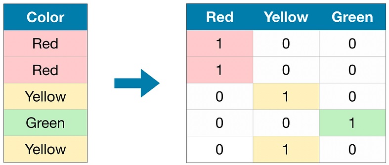
This approach lets us remove any notion of ordinality between the categories and thus we can represent them as independent and distinct features.

One way to do that is to add the following to the script:

It’s worth noting that the seemingly odd function name “get_dummies” does actually have a semantic relation to one-hot encoding. The term “dummies” is derived from the concept of creating “dummy variables” or “indicator variables” to represent categorical data as binary values during the process of encoding.

The output will be this:

      It  absolutely     is  necessary
0   True       False  False      False
1  False       False   True      False
2  False        True  False      False
3  False       False  False       True

What this code does is take the “Word” column of the DataFrame and returns a new DataFrame with the one-hot encoded representation of the categorical data. Each category will have its own column and the values in each row will be binary (1 or 0) to indicate the presence or absence of that category.

In Python, the boolean values True and False are internally represented as integers, where True is equivalent to 1 and False is equivalent to 0. If you wanted to convert the boolean values to integers, you can do that by changing the code we just added accordingly:

That would get you the following:

   It  absolutely  is  necessary
0   1           0   0          0
1   0           0   1          0
2   0           1   0          0
3   0           0   0          1

This now makes the binary nature of the contents a little more clear.

Make sure you see why using one-hot encoding like this helps to avoid the problem of fictitious ordering.

The reason is because the encoding explicitly represents each category as a separate binary column and that removes any unintended ordinal relationship between the categories. This approach helps to guide a neural network to treat each category as an independent and distinct feature.

As you can probably imagine, this particular DataFrame-based visualization could be a little harder to reason about if we applied it to the entire set of tokens in our text.

What this hopefully did, however, was give you one more way to conceptualize the one-hot encoding concept we’ve been working with in the previous post. This also gave you a way to see a potential problem inherent in the idea of assuming ordering where there is none.

Yet what happens when the ordering does actually matter?

Meaning of Data

In the encoded_text list, each element represents a numerical identifier corresponding to a specific token, which in our case is an individual character since that’s how we tokenized. These numerical identifiers are assigned based on a sorted set of unique tokens, ensuring a consistent and specific ordering. In this case, the tokens are sorted by punctuation, uppercase letters, and then lowercase letters, establishing a meaningful numerical relationship between the tokens.

That’s what we did in the last post. As we just talked about here, since the numerical identifiers are represented as integers, the encoded_text list appears to have a categorical scale. In a categorical scale, each numerical value represents a distinct category with no inherent order or ranking.

This is appropriate in the context of text classification, where the general goal is to provide a numerical representation of different tokens without implying any meaningful ordering among them.

But, at this point, you might be wondering something. If the tokens have no inherent ordering but human language does have ordering, then how can this representation be used by a learning model to actually, you know, learn?

While it’s true that the numerical representation of tokens in the encoded_text list doesn’t inherently capture the sequential information present in human language, the order of tokens is preserved in the data preparation and modeling process.

What that means is that when we feed the list into a machine learning model, we typically use methods that explicitly consider the sequential nature of language, which is what the Transformer-based models we’ll be looking at do.

That’s what we’ll get into as we get further into these posts. But I want to make sure this is really clear.

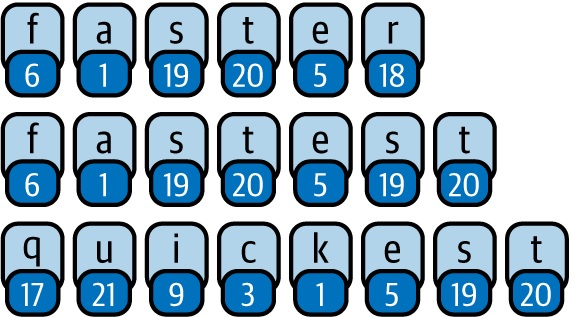
So let’s consider one of these examples:

 f  a  s  t  e  r
 6  1 19 20  5 18

Each element in the encoded list (the numbers) do not relate to each other but they do relate to each other when translated back to their token. So, yes, 6 and 1 and 19 have no relation to each other. But when mapped back to “f”, “a”, and “s” they do.

This demonstrates the purpose of encoding tokens as numerical identifiers. It allows us to represent text data in a format that can be processed by machine learning models effectively, even though the individual numerical identifiers themselves don’t hold any inherent meaning or relationship.

The power of Transformer-based models lies in their ability to learn meaningful patterns and relationships between the tokens using various methods — which you’ll hear called things like self-attention and positional encoding — regardless of the initial numerical representations.

Operations on Data

One consequence of the numerical identifiers in the encoded_text having no meaningful relationship is that performing arithmetic operations like addition or subtraction on them wouldn’t yield any meaningful result in the context of the original tokens.

For example, adding two numerical identifiers from the list would just create a new numerical identifier that doesn’t correspond to any real token in the data. The result is essentially meaningless and not interpretable in the context of the original text. To illustrate this point, let’s say you have the following numerical identifiers:

[2, 5, 7]

Adding 2 + 5 would result in 7. However, 7 doesn’t correspond to any real token in the data; it’s just another numerical identifier in the categorical scale. And adding 7 + 2 would result in 9 and that doesn’t correspond to anything in the data set at all.

This issue is exactly what we just discussed with the Pandas visualization of the one-hot encoding. In both cases, the numerical representations (IDs in Pandas or numerical IDs in our encoded_text) don’t convey any ordinal or meaningful relationship between the categorical entries (tokens).

Thus, performing operations on these numerical identifiers would lead to misinterpretations and incorrect conclusions. But … wait. You might wonder: “Why would I be performing arithmetic operations on this stuff anyway?”

And that’s a great question. In the context of language models and natural language processing, performing arithmetic operations like addition or subtraction on numerical identifiers of tokens generally isn’t a typical use case. Language models primarily deal with processing and understanding natural language text rather than performing numerical computations related to it.

Yet there are cases where such operations are relevant. One such is the one-hot encoding we’ve been talking about. For example, consider the following one-hot encoded vectors representing the tokens “absolutely” and “necessary”:

"absolutely": [0, 1, 0, 0, 0]
"necessary":  [0, 0, 0, 1, 0]

If we were to perform element-wise addition of these one-hot encodings, we would end up with this:

"absolutely" + "necessary": [0, 1, 0, 1, 0]

In this case, the resulting one-hot encoding tells us that both “absolutely” and “necessary” co-occur in the original text. But consider this:

"absolutely": [0, 1, 0, 0, 0]
"necessary":  [0, 0, 0, 0, 0]

"absolutely" + "necessary": [0, 1, 0, 0, 0]

The resulting one-hot encoding indicates that “absolutely” and “necessary” do not co-occur in the same text, as the latter token’s vector is all zeros.

There’s something you should start to notice with my examples. We’re still talking about character level tokenization but I’m showing you a whole lot of things with words. Keep that in mind since I’m taking you down a particular path here.

Back to Tensors

We still want to do the one-hot encoding but not for visualization purposes like we did in the previous post or even with Pandas above. Rather, we want to do it for execution purposes.

First go ahead and get rid of all the Pandas material from your script. And let’s use PyTorch for our tensor encoding.

pip install torch

To follow along, you’ll need the following imports:

The torch.nn module is a core module within the PyTorch library that provides a set of classes for building and training neural networks, hence the “nn.” Essentially the module defines a collection of pre-implemented layers and network architectures.

The torch.nn.functional module is a subset that contains a collection of functions for building neural networks that perform specific mathematical operations, one of those being the one-hot encoding we’ve been talking about.

Now add the following code to your script:

Let’s talk about what we’re doing here.

First, we’re converting the encoded_text list, which contains our numerical identifiers for each token in the text, into a PyTorch tensor, which essentially means a multi-dimensional array. Then we’re creating one-hot encodings for each element in the input_ids tensor that we just created.

The resulting tensor will have the shape of [seq_length, vocab_size]. Here the first element is the length of the input text — the number of characters in the text — and the second is the number of unique characters in the text. You can actually see that shape if you want:

The output is:

torch.Size([299, 29])

The first dimension (299) represents the sequence length of the input text. In this case, the sequence length is 299, which means our original text was tokenized into 299 individual characters.

The second dimension (29) represents the size of the vocabulary or the number of unique characters in the tokenized text. In this case, there are 29 unique characters.

This should seem very familiar to you in terms of what we did in the previous post. But there we did everything by coding it ourselves; here we’re using PyTorch to assist us.

There’s something worth calling out here in the above code.

That num_classes parameter is really important. Setting this is crucial to make sure that the resulting one-hot vectors have the correct length (read: size) equal to the vocabulary size. If we don’t specify this parameter, the one-hot vectors may end up being shorter than the vocabulary size. That can lead to incorrect results or errors.

The F.one_hot() function I’m using here takes the input tensor of integer values — representing the numerical identifiers — and converts it to one-hot encoded tensors. Let’s take a look at the first vector.

That will give the following output:

Token: I
Tensor index: 5
One-hot: tensor([0, 0, 0, 0, 0, 1, 0, 0, 0, 0, 0, 0, 0, 0, 0, 0, 0, 0, 0, 0, 0, 0, 0, 0, 0, 0, 0, 0, 0])

The first statement shows the first token in the tokenized text, which is “I”. The token “I” corresponds to the first character in the original text.

The second line shows the corresponding numerical identifier for the token “I” in the model input. The numerical identifier for “I” is 5, indicating that “I” is the fifth unique token in the tokenized text.

The last line shows the one-hot encoded vector for the token “I” in the one-hot encodings tensor. Since the numerical identifier for “I” is 5, the one-hot encoded vector will have a “1” at the fifth position (assuming 0-based indexing) and “0” in all other positions.

Again, all of this should seem very familiar from the work we did in the first post.

The Meaning of Our Text

Let’s keep in mind an important point here: in our example so far we’ve been using character-level tokenization.

This means the text is broken down into individual characters and each character is thus treated as a separate token. Now here’s something critical to note: the process of character-level tokenization ignores any linguistic or semantic structure present in the text and treats the entire string as a sequential stream of characters.

This means character-level tokenization doesn’t take into account word boundaries or syntactic structure. Instead it just treats every character as a separate unit, regardless of whether that character forms a meaningful word or not.

Maybe this sounds terrible but this approach can be useful in certain scenarios, such as handling languages with complex word formations or when maintaining fine-grained details at the character level is important.

While the approach can be useful, character-level tokenization is generally not ideal for tasks that rely on understanding higher-level linguistic patterns, such as sentence meaning or word relationships. This is, in fact, exactly what we’re going to be focusing on with some upcoming examples, such as emotion sentiment. In these kinds of cases, tokenizing at the word or subword level might be more appropriate to capture the meaningful units in the text.

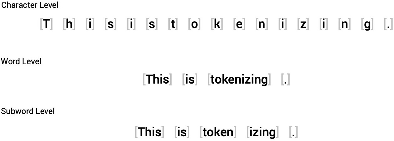
What this means is that we instead want some structure of the text to be preserved during the tokenization step. This takes us right into another of the tokenization strategies, which is word tokenization.

Element-wise addition, like I showed earlier, can be performed on any encoded text. However, doing so on character tokenized text might be significantly more difficult and less meaningful compared to word tokenized text, hence our desire to switch strategies.

Tokenize By Word

Instead of splitting the text into characters as we did previously, we can instead split it into words and map each word to an integer. Using words from the outset, rather than just characters, would allow the model to skip the step of learning words from characters. That would certainly reduce the complexity of the training process.

One simple class of word tokenizers uses whitespace to tokenize the text. We can do this very simply. First let’s just entirely reset our script logic like this:

The output here is:

['It', 'is', 'absolutely', 'necessary,', 'for', 'the', 'peace', 'and', 'safety', 'of', 'mankind,', 'that', 'some', 'of', "earth's", 'dark,', 'dead', 'corners', 'and', 'unplumbed', 'depths', 'be', 'let', 'alone;', 'lest', 'sleeping', 'abnormalities', 'wake', 'to', 'resurgent', 'life,', 'and', 'blasphemously', 'surviving', 'nightmares', 'squirm', 'and', 'splash', 'out', 'of', 'their', 'black', 'lairs', 'to', 'newer', 'and', 'wider', 'conquests.']

From here we could take the exact same steps we took for the character tokenizer to map each word to a numeric identifier. However, before we go down that route, there’s already one potential problem with this tokenization scheme. See if you can spot it in the output above.

Punctuation isn’t accounted for. So we see “necessary,” and “conquests.” — with the punctuation as part of the token. So what the above output shows is that these words with the punctuation are treated as a single token. What do we do about that?

Some word tokenizers do have extra rules for punctuation which can take care of that problem. You can also apply certain techniques like stemming or lemmatization. These technique normalize words to their stem. So, as an exmaple, the words “argue”, “argues”, “arguing”, and “argued” could all be normalized to their base form “argue”. Similarly, the words “play”, “plays”, “played”, and “playing” could be normalized to their base form “play”.

Obviously there’s yet another potential problem that rears its head here, though. Any such changes like these clearly cause some information to be lost from the text. Whether what’s lost matters or not is highly context-dependent.

Our example text is fairly small but it’s not an inconsequential bit of vocabulary. And certainly we’ll have a lot more vocabulary to potentially deal with in our later examples around movie reviews, social media emotions and scientific claims.

Scaling Up to Lots of Text

Consider this logistic: a large vocabulary implies a high number of unique words in the dataset. When using word tokenization, each word becomes a separate token. Thus the size of the vocabulary directly affects the number of unique tokens. This, in turn, increases the number of parameters required for the neural network. That can lead to memory and computational inefficiencies.

Keep in mind the dimensions we talked about in the previous post. Let’s say that in a given text, we have one thousand unique words. That would mean we have a 1,000-dimensional space. So what we usually do is try to compress those dimensions a bit.

Yet this leads us into an interesting balancing act between character tokenization and word tokenization.

Character tokenization retains all the input information as each character is treated as a separate token. However, it may lose some higher-level linguistic meaning and context since it doesn’t inherently recognize word boundaries or meaningful word units.

On the other hand, word tokenization captures more meaningful linguistic structures, allowing the model to retain more semantic meaning, word relationships, and context. However, it may lose some of the fine-grained details and specific character-level information because words are treated as separate units.

It seems we’re caught between the proverbial “rock and a hard place.” What we want is a middle ground.

Tokenize By Sub-Word

Subword tokenization techniques work by dividing words into smaller subword units. Such units refer to things like prefixes, suffixes, and root words.

• Consider the word “unhappy”. Here the prefix would be “un-” and the root would be “happy”. There is no suffix.

• Consider the word “reacted”. Here the root is “react” and the suffix is “-ed”. There is no prefix.

• Consider the word “misunderstood”. Here the prefix is “mis-“, the root is “understand” and the suffix is “-ood”.

The division into subword units is learned from the statistical properties of the text data during the training process.

To make that point clear, patterns and frequencies are observed in the training text data. During the training process, the subword tokenization algorithm analyzes the text and looks for common subword units — like those prefixes, suffixes, and root words — that occur frequently in the text. The algorithm learns the statistical distribution of these subword units and uses that information to split words into meaningful subword pieces.

The practical upshot of all this is that the tokenization process tries to find the most effective subword units that help capture meaningful linguistic structures and reduce the size of the vocabulary.

To keep this really simple, let’s just consider this text: “I like apples, apple pie, and apple juice.” Here’s what simple word tokenization would get us:

['I', 'like', 'apples,', 'apple', 'pie,', 'and', 'apple', 'juice.']

Here’s what subword tokenization would get us:

['I', 'like', 'appl', '##es', ',', 'apple', 'pie', ',', 'and', 'juice', '.']

In this example, the subword tokenization process has effectively reduced the vocabulary size by breaking down the word “apples” into “appl” and “##es” and the word “apple” is preserved as a separate subword unit. The subword tokenization resulted in a list of eleven tokens, while the word-level tokenization had a list of seven tokens, showcasing the reduction in vocabulary size.

Thus, in the context of tokenization, the word-level list should ideally have fewer items than the subword list. This difference intuitively reflects the reduction in vocabulary size achieved through subword tokenization.

By breaking down words into smaller subword units like this, subword tokenization can represent words more efficiently. It can also more effectively handle variations in word forms. That’s helpful for languages with rich morphology, compound words, and various inflections.

Learning From the Text

A key point to take from the above is that the tokenization strategy is learned from the data rather than being pre-defined.

This allows the tokenization to adapt to the specific characteristics of the language and the text used for pre-training. This makes it possible for the tokenizer to be more effective at capturing meaningful units for downstream language tasks.

What you should be taking from this is that the learning process involves a mix of statistical analysis and algorithms to determine the most appropriate tokenization strategy for the given text data.

We’ve been constructing our own strategies in these posts so far to focus on fundamentals but now we’re going to start using things as you will likely encounter them.

There are several subword tokenization algorithms that are commonly used in this context but let’s start with WordPiece. This is used by the BERT and DistilBERT tokenizers. RoBERTa uses a variant of the WordPiece tokenizer called the SentencePiece tokenizer.

Remember that our plan is to use Transformer models here and the Transformers library provides an AutoTokenizer class. This class allows you to quickly load a tokenizer that’s associated with a pre-trained model. You’ll need to install the transformers library.

pip install transformers

Let’s start over with a brand new script just so we can focus on the new stuff.

Up to this point we’ve sort of been just building our own tokenizers. But now we’re getting a little more official and using the tokenizer provided by a pre-trained model.

If you haven’t previously run with this checkpoint, the above logic will download the necessary components to your machine.

You can check some key attributes of the tokenizer we’re using. For example:

This will output 30522. This value represents the size of the vocabulary used by the tokenizer. In this case, what this tells us is that the tokenizer can map 30,522 different tokens (words or subwords) to unique numerical identifiers. You can also do this:

This will output 512. This value represents the maximum length of the input that the model can accept. In this case, what this means is that the maximum number of tokens in whatever input text is will be limited to 512. If the input text exceeds this length, it will be truncated. Finally, try this:

You will see this output:

['input_ids', 'attention_mask']

This value is a list of input names that the model can accept. In this case, the model expects two inputs. The “input_ids” are the numerical identifiers representing the tokens in the text. The “attention_mask” is used to indicate which tokens the model should pay attention to during processing.

In our code, I’m calling the from_pretrained() method, providing the ID of a model. Thus the code is loading the tokenizer for DistilBERT. If you wanted to use BERT, you would do this instead:

Likewise, for RoBERTa you could do this:

The output for the above attributes would be mostly the same for BERT although the model_input_names will output this:

['input_ids', 'token_type_ids', 'attention_mask']

Also, if you use RoBERTa, you’ll find the vocabulary size is 50,265.

Each of those strings — distilbert-base-uncased, bert-base-uncased, and roberta-base — is also referred to as a checkpoint in the context of the Transformers library.

As mentioned in the previous post, in the context of learning models, a checkpoint refers to a snapshot of the model’s parameters at a particular point during training.

Checkpoints are often saved periodically during training and they can be used to resume training from that point or to make predictions using the saved model.

In the case of the Transformers library, the pre-trained models are provided as checkpoints that are pre-trained on a large amount of text data for a specific natural language processing task, such as language modeling or question answering or, as in our case, text classification.

Encoding Our Text

As we did with our running example so far, let’s use the tokenizer provided on the text.

You get the following output:

{'input_ids': [101, 2009, 2003, 7078, 4072, 1010, 2005, 1996, 3521, 1998, 3808, 1997, 14938, 1010, 2008, 2070, 1997, 3011, 1005, 1055, 2601, 1010, 2757, 8413, 1998, 4895, 24759, 25438, 2098, 11143, 2022, 2292, 2894, 1025, 26693, 5777, 28828, 5256, 2000, 24501, 27176, 2166, 1010, 1998, 1038, 8523, 8458, 6633, 13453, 6405, 15446, 5490, 10179, 10867, 1998, 17624, 2041, 1997, 2037, 2304, 21039, 2015, 2000, 10947, 1998, 7289, 9187, 2015, 1012, 102], 'attention_mask': [1, 1, 1, 1, 1, 1, 1, 1, 1, 1, 1, 1, 1, 1, 1, 1, 1, 1, 1, 1, 1, 1, 1, 1, 1, 1, 1, 1, 1, 1, 1, 1, 1, 1, 1, 1, 1, 1, 1, 1, 1, 1, 1, 1, 1, 1, 1, 1, 1, 1, 1, 1, 1, 1, 1, 1, 1, 1, 1, 1, 1, 1, 1, 1, 1, 1, 1, 1, 1, 1]}

Just as with character tokenization, you can see that the words have been mapped to unique integers.

What we get here is a list of integers representing the tokenized input text. Each integer corresponds to the ID of a token in the vocabulary of the pre-trained model.

The list starts with 101 and ends with 102, which are special tokens indicating the beginning and end of the input sequence, respectively. The numbers in between are the token IDs for the individual words in the input text.

The attention mask is a list of integers (only 0 or 1) indicating whether each token in the input_ids list should be attended to or not. In this case, all tokens have an attention mask of 1, indicating that they are all valid tokens and the model should thus pay attention to them.

Now that we have the this numeric list, we could, if we needed to, convert them back into tokens by using a method provided by the tokenizer.

If you try that out, you’ll get the following output:

['[CLS]', 'it', 'is', 'absolutely', 'necessary', ',', 'for', 'the', 'peace', 'and', 'safety', 'of', 'mankind', ',', 'that', 'some', 'of', 'earth', "'", 's', 'dark', ',', 'dead', 'corners', 'and', 'un', '##pl', '##umb', '##ed', 'depths', 'be', 'let', 'alone', ';', 'lest', 'sleeping', 'abnormalities', 'wake', 'to', 'res', '##urgent', 'life', ',', 'and', 'b', '##las', '##ph', '##em', '##ously', 'surviving', 'nightmares', 'sq', '##ui', '##rm', 'and', 'splash', 'out', 'of', 'their', 'black', 'lair', '##s', 'to', 'newer', 'and', 'wider', 'conquest', '##s', '.', '[SEP]']

Notice those special [CLS] and [SEP] tokens that have been added to the start and end of the sequence. In the previous output, we saw that the input_ids list started with 101 and ended with 102. These correspond to special tokens known as [CLS] and [SEP], respectively.

You’ll also notice the tokens have each been lowercased. Remember that we’re using the “distilbert-base-uncased” model. The “uncased” part in the model name indicates that the model is trained on uncased text, meaning that all text is converted to lowercase during training.

As a result, when you use this tokenizer to tokenize and encode text, it automatically converts all the input text to lowercase. This is done to make the model more robust to case variations and to reduce the size of the vocabulary, as it treats uppercase and lowercase versions of the same word as the same token.

We can see that “resurgent” has been broken into two: ‘res’ and ‘##urgent’. Notice how “unplumbed” has become ‘un’, ‘##pl’, ‘##umb’, ‘##ed’.

You might wonder why it does this, particularly for those words. This type of tokenization can help models like BERT, DistilBERT, and RoBERTa handle rare or out-of-vocabulary words more effectively since the subword units can be shared between different words. It also allows for better handling of morphologically complex languages where words can have a variety of prefixes and suffixes.

The ## prefix means that the preceding string is not whitespace; any token with this prefix should be merged with the previous token when you convert the tokens back to a string. The AutoTokenizer class has a particular method for doing just that, so let’s apply it to our tokens:

Nothing terribly surprising here. That gets you:

[CLS] it is absolutely necessary, for the peace and safety of mankind, that some of earth ' s dark, dead corners and unplumbed depths be let alone ; lest sleeping abnormalities wake to resurgent life, and blasphemously surviving nightmares squirm and splash out of their black lairs to newer and wider conquests. [SEP]

But you might notice a few differences there. Do you see them?

Notice how “earth’s” became “earth ‘ s” and the semicolon has spaces between it.

The reason for this is that the tokenizer treats certain punctuation and special characters in a specific way during tokenization.

So, in this case, “earth’s” became “earth ‘ s” because the tokenizer tokenizes the possessive apostrophe (‘) as a separate token, and it adds spaces around it to distinguish it from the adjacent words. This is to ensure that the tokenization process is reversible, and the original text can be accurately reconstructed from the tokens.

In the case of the semicolon “;”, the tokenizer also adds spaces around some punctuation marks to separate them as individual tokens. This is again done to preserve the ability to reconstruct the original text from the tokens.

Wrapping Up

Okay, this is probably enough of digging in to the fundamentals. What I hope you saw through these first two posts is we explored the ideas by writing our own tokenizer and encoder and then looked at doing the same thing more officially with a pre-trained model that provides a tokenizer and encoder.

What this does is now set us up to actually look at the idea of our data a bit more broadly. I’ve been using a simple paragraph of text. Yet now we have to get into the idea of datasets, which we’ll tackle in the next post.