Let’s start this “Thinking About AI” series by thinking about the idea of classifying text. Classifying, broadly speaking, relates to testing quite well. This is because, at its core, the idea of classification focuses on categorization of data and decision making based on data. More broadly, as humans, we tend to classify everything by some categories.

This series has its start in the framing post Thinking About AI. Reading that is not necessary, however, for diving in to this post.

The Basic Plan

One of the most common areas that people get started on in relation to text classification is referred to as sentiment analysis. The goal with this concept is to determine the polarity of some text. Here “polarity” refers to the emotional or sentimental orientation expressed in a given text, usually framed as positive, negative or neutral.

The word “polarity” itself is derived from the concept of polarity in physics, which refers to the positive or negative charge of a magnetic or electric field. The analogy may seem stretched but the general idea is that of a relationship between two opposite characteristics or tendencies.

There’s another context to consider which is known as claim verification or fact-checking. Here the focus is to determine whether a claim is supported or contradicted by any provided evidence in a given text. In this context you don’t really deal with polarity at all but rather the relationship between a claim and evidence provided to support that claim.

I’m going to explore both contexts in this series so that you have some familiarity with the distinction. To do that will require some data that provides a whole bunch of text related to the type of classification that you’re dealing with.

Much like in the wider testing world, your data strategy is crucial. One of my focal points in this series will be looking at various sets of data and showing you how we can reason about those data sets in the context of text classification.

So that’s the broad plan. But we need a context to carry out that plan in.

The Basic Context

Rather than have one specific example that will serve as the throughline for these posts, I’m going to explore multiple examples here. All of the examples I provide will be focused on the idea of text classification and, specifically, about sending text into a learning model so that the model can make relevant predictions about the text.

I’ll look at tasks such as learning sentiment from movie reviews, learning emotional stances form social media posts, and learning relationships between supported and contradicted scientific claims.

Along with that, I’ll talk about handling text classification using various pre-trained models, specifically BERT, DistilBERT and RoBERTa. Switching between those models is as simple as changing what’s called the checkpoint that refers to each model.

A “checkpoint” refers to a specific saved instance of a pre-trained model, containing its learned parameters and overall architecture. This saved instance can be easily loaded and utilized for various tasks like text classification.

Think of the checkpoint as analogous to the state of a model at a specific point in time during its training or after being trained.

So our context is that we’re looking into specific data that we can feed to various models that will allow us to classify text along some spectrum. The first part of our focus will be on how to feed data to our models. The second part of our focus will be on what the model does once it has been fed some data.

I’m going to assume very little pre-existing knowledge here and so I’m going to start off by exploring some fundamentals. Then I’ll apply those fundamentals to some public datasets based on the tasks I mentioned above. This approach should give you a good mix of theory and practice, but skewing more towards practice.

The Basis of Classification

Before we dig into some specific use cases and datasets, let’s take a step back and actually look at how data gets into these models by using a pedagogical approach that’s highly reductionist in nature. By this I mean I’m going to show you at a very granular level what a lot of the tooling out there does for you automatically.

I highly recommend you create a Python script and work along with me but I will show all output here so that you can follow along even if you don’t use the code.

I tend to show Python a lot because it’s often the easiest ecosystem for people to get started in. But you certainly can achieve anything I show in various languages.

Let’s start with some example text data.

That statement comes from H.P. Lovecraft’s At the Mountains of Madness, if you’re curious.

So let’s say we want to classify that text.

Classifying Text via Transformers

Ultimately we’re going to use Transformer models for this kind of task. For now just understand “Transformer model” as a type of machine learning algorithm designed to comprehend and process human language, simulating how a human would understand and interpret textual data.

What this means is that we want to pass our text into a Transformer model.

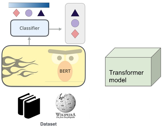
Well, actually, that’s not quite accurate. These models can’t just receive raw strings of text like the above as input. We need to do some tokenizing and encoding.

In the context of Transformer models, tokenizing refers to breaking down a string of text into some atomic units, which are used as input to the model. Not just any atomic units, however. But rather atomic units that are specifically used in the model.

The specific units used in a given model depends on the tokenization strategy used by the model in question. We’re going to look at those strategies in these posts, which tend to fall under broad categories of character tokenization, word tokenization and sub-word tokenization.

Once the tokenizing is done, then encoding takes place. This is where the tokenized atomic units are converted into numbers.

Much like tokenizing, different models can have distinct strategies for encoding tokenized text. Such strategies go by names like one-hot encodings, word embeddings, positional encodings and so on. We’re going to look at one-hot encodings in particular when we get to encoding our data.

Initial Steps

So let’s set the stage here. To start off, we’re going to tokenize (by character) and encode (via one-hot).

What this will do is give us the process for how we can turn text, like our above example text, into an encoded representation that can be passed to a Transformer-based learning model. This simple text example will serve as the basis for understanding how all of this works even with much larger text data sets.

Tokenize By Character

Let’s first handle the tokenizing of our text by individual character.

This strategy is pretty much exactly what it sounds like: we literally feed each character of the text individually to the model. To be more accurate, we do that after those characters have been encoded. As stated above, encoding is always necessary and we’ll come to that later. For now, let’s just handle the tokenizing part. You can add the following to the script:

This is the output:

['I', 't', ' ', 'i', 's', ' ', 'a', 'b', 's', 'o', 'l', 'u', 't', 'e', 'l', 'y', ' ', 'n', 'e', 'c', 'e', 's', 's', 'a', 'r', 'y', ',', ' ', 'f', 'o', 'r', ' ', 't', 'h', 'e', ' ', 'p', 'e', 'a', 'c', 'e', ' ', 'a', 'n', 'd', ' ', 's', 'a', 'f', 'e', 't', 'y', ' ', 'o', 'f', ' ', 'm', 'a', 'n', 'k', 'i', 'n', 'd', ',', 't', 'h', 'a', 't', ' ', 's', 'o', 'm', 'e', ' ', 'o', 'f', ' ', 'e', 'a', 'r', 't', 'h', "'", 's', ' ', 'd', 'a', 'r', 'k', ',', ' ', 'd', 'e', 'a', 'd', ' ', 'c', 'o', 'r', 'n', 'e', 'r', 's', ' ', 'a', 'n', 'd', ' ', 'u', 'n', 'p', 'l', 'u', 'm', 'b', 'e', 'd', ' ', 'd', 'e', 'p', 't', 'h', 's', ' ', 'b', 'e', ' ', 'l', 'e', 't', ' ', 'a', 'l', 'o', 'n', 'e', ';', 'l', 'e', 's', 't', ' ', 's', 'l', 'e', 'e', 'p', 'i', 'n', 'g', ' ', 'a', 'b', 'n', 'o', 'r', 'm', 'a', 'l', 'i', 't', 'i', 'e', 's', ' ', 'w', 'a', 'k', 'e', ' ', 't', 'o', ' ', 'r', 'e', 's', 'u', 'r', 'g', 'e', 'n', 't', ' ', 'l', 'i', 'f', 'e', ',', ' ', 'a', 'n', 'd', ' ', 'b', 'l', 'a', 's', 'p', 'h', 'e', 'm', 'o', 'u', 's', 'l', 'y', 's', 'u', 'r', 'v', 'i', 'v', 'i', 'n', 'g', ' ', 'n', 'i', 'g', 'h', 't', 'm', 'a', 'r', 'e', 's', ' ', 's', 'q', 'u', 'i', 'r', 'm', ' ', 'a', 'n', 'd', ' ', 's', 'p', 'l', 'a', 's', 'h', ' ', 'o', 'u', 't', ' ', 'o', 'f', ' ', 't', 'h', 'e', 'i', 'r', ' ', 'b', 'l', 'a', 'c', 'k', ' ', 'l', 'a', 'i', 'r', 's', ' ', 't', 'o', ' ', 'n', 'e', 'w', 'e', 'r', 'a', 'n', 'd', ' ', 'w', 'i', 'd', 'e', 'r', ' ', 'c', 'o', 'n', 'q', 'u', 'e', 's', 't', 's', '.']

Okay, so that’s some progress. That said, we still have text. Now it’s just broken up text. But remember that our model will expect — in fact, require — each character to be converted to an integer. This is where encoding comes in. Sometimes this process is referred to as numericalization.

The terms “encoding” and “numericalization” are often used interchangeably when discussing the process of converting tokenized text into numerical values. Both terms refer to the essential step of preparing the text input for further processing by the model.

Here’s a crucial point that sometimes gets left off: this process of encoding is based on the vocabulary that’s being dealt with.

Generate a Vocabulary

Before we do any encoding, we want to establish a predefined vocabulary. Specifically, I want to establish the predefined vocabulary from the tokenized text.

Here a “predefined vocabulary” consists of all the characters that will be encountered during the tokenization process. This obviously refers to the letters but it also refers to the punctuation marks, spaces, and any other symbols that appear in the text.

The term “predefined” here really just means “defined in the text” as opposed to something that’s being referenced outside the text. It’s “predefined” as far as the model is concerned.

Add the following to the script:

By converting the tokenized text into a set and then sorting it, what we’re doing is ensuring that the predefined vocabulary contains a unique and ordered list of characters present in the tokenized text. The output will be the following:

[' ', "'", ',', '.', ';', 'I', 'a', 'b', 'c', 'd', 'e', 'f', 'g', 'h', 'i', 'k', 'l', 'm', 'n', 'o', 'p', 'q', 'r', 's', 't', 'u', 'v', 'w', 'y']

This list represents all the unique characters found in the given text. This list will be used to create a mapping between characters and corresponding numeric indices, which is essential for encoding the text and feeding it into a Transformer model.

You can see that the sorting process follows a default behavior where characters are ordered based on their ASCII values. In this case, the punctuation symbols have lower ASCII values compared to uppercase letters, and uppercase letters have lower ASCII values compared to lowercase letters.

To give all this a name, what we just did here was vocabulary generation.

Encode By Character

Our next goal is to make sure that each unique token is replaced with a unique integer. Here “token” refers to whatever unit we’re talking about which, in this case, would be the individual characters.

Here again I’ll remind that Transformer models like BERT, DistilBERT and RoBERTa can’t receive raw text, even when broken down into atomic units. Instead, these models assume the text has been tokenized and encoded as numerical vectors.

When I say “numerical vector” what that refers to is a sequence of numerical values that are used to represent the tokenized text. These vectors are derived by mapping each token in the text to a unique integer value and then representing the sequence of these index values as a vector.

Okay, so why is it called a vector?

In mathematics, a vector is a mathematical object that represents both magnitude and direction. It has multiple components — points — along each dimension in a multidimensional space. Each component of the vector corresponds to a particular dimension in that space.

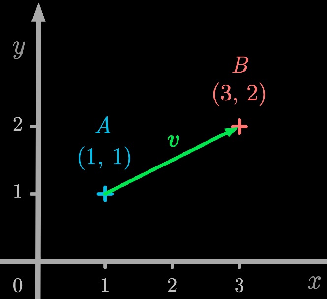
The numerical vector used to represent tokenized text is conceptually similar to a mathematical vector in that it’s a sequence of values. Each value in the numerical vector represents the index of a token in the text. Thus the dimension in this context is not spatial but rather positional within the sequence of tokens. So instead of something like this:

We have something more like this:

Thus while the concept of a numerical vector representing tokenized text is related to a mathematical vector, it doesn’t inherently have a spatial interpretation. Instead, it provides a structured way to encode sequential information.

But Why The Vocabulary Step?

You might wonder something at this point. Why don’t we just encode the original tokenized text? Why did we do vocabulary generation in order to encode that instead?

Encoding the original tokenized text directly without vocabulary generation can be done. However, doing that might not be the most efficient or practical approach. This is particularly the case when you’re dealing with large datasets or extensive vocabularies. So one of the key factors here in this consideration is size of data.

In natural language, the number of unique tokens — characters, words, subwords — can obviously be quite large. If you encode the original tokenized text directly, you might end up with a massive data structure and that can be computationally expensive and memory-intensive.

Obviously that’s not the case with our small text being used here but the point still stands. Thus our interim vocabulary generation step allows us to map all of the tokens to a smaller, fixed-size vector representation, making it more manageable for the model.

Dimensionality

Before moving on to the encoding step proper, let’s unpack this idea of dimensions a bit.

I like the idea of dimensional thinking. You can see my post on “The Dimensionality of Testing” as well as my ramblings on whether testing is geometry or topology.

With what we’ve done above, we’re saying that each unique token will be mapped to a unique integer value. The resulting numerical vector will represent the sequence of these index values, capturing the entire structure of the tokenized, vocabulary-generated text.

• The dimensionality of the tokenized text is 299.
• The dimensionality of the vocabulary-generated text is 29.

Remember that the tokenized text is the number of tokens in the input text. For character-level tokenization, the dimensionality is equal to the number of characters in the text. Thus each token (character) represents a separate dimension in the tokenized text.

The vocabulary-generated text is the number of unique tokens in the input text. Each unique token (character) represents a separate dimension in the vocabulary-generated text.

Encoding Along the Dimension

I said that we want to make sure that each unique token is replaced with a unique integer. So let’s do exactly that.

Keep in mind that when you numericalize text by assigning integer values to characters (or tokens), each occurrence of a specific character will be mapped to the same integer value. In other words, all instances of a particular character token will be represented by the same unique integer in the numerical vector.

Thus if it’s the case that the uppercase letter “I” gets mapped to the integer 5, all instances of the uppercase letter “I” will be mapped to 5.

Let’s add some logic to our script:

This gives us a mapping from each character in our vocabulary to a unique integer. You’ll get the following output:

{' ': 0, "'": 1, ',': 2, '.': 3, ';': 4, 'I': 5, 'a': 6, 'b': 7, 'c': 8, 'd': 9, 'e': 10, 'f': 11, 'g': 12, 'h': 13, 'i': 14, 'k': 15, 'l': 16, 'm': 17, 'n': 18, 'o': 19, 'p': 20, 'q': 21, 'r': 22, 's': 23, 't': 24, 'u': 25, 'v': 26, 'w': 27, 'y': 28}

This dictionary maps each unique character from the vocabulary to a corresponding integer index.

What we can do now is take our numericalized text and transform our tokenized text to a list of integers. Here’s a simple way to do that:

Here I’m just using a list comprehension to say that for each character token in the tokenized text, the corresponding numerical identifier from the numericalized text should be retrieved and added to the list of what will be our encoded text. The output is this:

[5, 24, 0, 14, 23, 0, 6, 7, 23, 19, 16, 25, 24, 10, 16, 28, 0, 18, 10, 8, 10, 23, 23, 6, 22, 28, 2, 0, 11, 19, 22, 0, 24, 13, 10, 0, 20, 10, 6, 8, 10, 0, 6, 18, 9, 0, 23, 6, 11, 10, 24, 28, 0, 19, 11, 0, 17, 6, 18, 15, 14, 18, 9, 2, 24, 13, 6, 24, 0, 23, 19, 17, 10, 0, 19, 11, 0, 10, 6, 22, 24, 13, 1, 23, 0, 9, 6, 22, 15, 2, 0, 9, 10, 6, 9, 0, 8, 19, 22, 18, 10, 22, 23, 0, 6, 18, 9, 0, 25, 18, 20, 16, 25, 17, 7, 10, 9, 0, 9, 10, 20, 24, 13, 23, 0, 7, 10, 0, 16, 10, 24, 0, 6, 16, 19, 18, 10, 4, 16, 10, 23, 24, 0, 23, 16, 10, 10, 20, 14, 18, 12, 0, 6, 7, 18, 19, 22, 17, 6, 16, 14, 24, 14, 10, 23, 0, 27, 6, 15, 10, 0, 24, 19, 0, 22, 10, 23, 25, 22, 12, 10, 18, 24, 0, 16, 14, 11, 10, 2, 0, 6, 18, 9, 0, 7, 16, 6, 23, 20, 13, 10, 17, 19, 25, 23, 16, 28, 23, 25, 22, 26, 14, 26, 14, 18, 12, 0, 18, 14, 12, 13, 24, 17, 6, 22, 10, 23, 0, 23, 21, 25, 14, 22, 17, 0, 6, 18, 9, 0, 23, 20, 16, 6, 23, 13, 0, 19, 25, 24, 0, 19, 11, 0, 24, 13, 10, 14, 22, 0, 7, 16, 6, 8, 15, 0, 16, 6, 14, 22, 23, 0, 24, 19, 0, 18, 10, 27, 10, 22, 6, 18, 9, 0, 27, 14, 9, 10, 22, 0, 8, 19, 18, 21, 25, 10, 23, 24, 23, 3]

So there’s our encoding! Essentially each token in our predefined vocabulary, by which is meant our original text, has been mapped to a unique numerical identifier consistent with the numericalization that we generated.

The length of the encoded_text list is 299, which matches the original token count of the tokenized text. This is expected because each character in the tokenized text is mapped to a unique integer from the numericalized_text dictionary and the resulting numerical vector (encoded_text) retains the same number of elements as the original tokenized text.

This is crucial. In fact, this is extremely crucial. The encoding process maintains the one-to-one correspondence between characters in the tokenized text and their integer representations in the numerical vector, ensuring that the structure and information in the text are preserved in the encoded form.

Equally crucial is you can see how many unique elements are in that above encoding. If you want to prove it yourself, go ahead and do this:

You’ll see the count is 29. That, too, makes sense. There were 29 unique categories of token.

Does It Make Sense?

Make sure you see what the code we just wrote is showing you. There are four distinct steps there: tokenization, vocabulary generation, numericalization, and encoding. Each is nicely encapsulated by one statement of logic.

Without the numericalization step, you would not have a proper numerical representation of the tokenized text. Instead, you would have a list of character tokens (raw text) that couldn’t be directly used as input for most machine learning algorithms.

Without the encoding step, you would simply be passing a mapping of unique tokens to integers to the model, which it would have no means of doing anything with.

Encoding as a Tensor

We’ve encoded our data into a one-dimensional numerical vector, where each integer represents the index of a unique token in the predefined vocabulary. Now we want to further process the numerical vector to create a binary tensor.

Each element in this tensor will be a binary value — 0 or 1 — indicating the presence or absence of a token in the input sequence.

Here I’m emphasizing the distinction between the numerical vector (a one-dimensional structure) and the binary tensor (a multi-dimensional structure).

Why a tensor specifically?

The term “tensor” is derived from mathematics, particularly from the field of linear algebra.

A tensor is effectively an array of elements arranged in a specific way, with respect to the number of indices required to access those elements. What this means is that a tensor can be thought of as a generalization of vectors and matrices to higher dimensions. Consider that a scalar value is a zero-dimensional tensor, whereas a vector is a one-dimensional tensor, and a matrix is a two-dimensional tensor.

All of the above in that visual are tensors. A scalar just happens to be a tensor of rank 0. A vector is a tensor of rank 1 and so on.

Our numerical vector that we just created can be represented as a one-dimensional tensor since it has only one dimension.

This process of encoding to a tensor is commonly used in natural language processing to represent categorical data, such as our tokenized and encoded text. Categorical data refers to a type of data that represents discrete, qualitative attributes or characteristics. These attributes are of two broad types: nominal or ordinal.

• Nominal data are variables that have no inherent order or ranking between categories. For example, “opportunity”, “risk” and “balanced” are nominal categorical variables.

• Ordinal data are variables that have an inherent ranking or order between categories. Good examples of ordinal categorical variables would be grades (A, B, C, D, and F), ratings (low, medium, or high), or some type of levels (beginner, intermediate, expert).

In the context of sentiment, terms like “negative,” “positive,” and “neutral” are not considered nominal data. Instead, they fall under the category of ordinal data because they can be ranked in a meaningful way. The same would apply to the terms “supported,” “contradicted,” and “undecided” in the context of claim verification.

Clearly our text is nominal data. The character tokens don’t have any inherent order or ranking; they’re simply unique symbols representing specific characters. There’s no natural progression or hierarchy among the characters.

Do you see an inherent problem in what I just said given the nature of text classification tasks? If so, you’re on your way to building some good instincts. This will come up again in the second post in this series.

Seeking Clarity on Dimensions

To make some of these points clear, let’s say we had this simple numerical vector:

[0, 1, 2, 3, 4, 5, 6, 7, 8, 9, 10, 11]

This is a one-dimensional tensor because it has one dimension, meaning one row or one axis. A binary vector representation of that would look something like this:

[[1, 0, 0, 0],
 [0, 1, 0, 0],
 [0, 0, 1, 0],
 [0, 0, 0, 1],
 [0, 0, 0, 1],
 [0, 0, 0, 1],
 [0, 0, 0, 1],
 [0, 0, 0, 1],
 [0, 0, 0, 1],
 [0, 0, 0, 1],
 [0, 0, 0, 1],
 [0, 0, 0, 1]]

This is a two-dimensional tensor because it has two dimensions, meaning rows and columns. Thus this structure can be seen as a multi-dimensional array. Seeing these structures as arrays can be really helpful, particularly in the programmatic context.

Seeking Simplicity with Dimensions

But why do we need our one-dimensional structure to become this two-dimensional structure?

The resulting two-dimensional tensor will contain what are called one-hot vectors for each token in the text. Each row will represent a token and the columns will indicate the presence or absence of the token’s integer value in the one-hot encoded form.

The name “one-hot” comes from the fact that in the vector, only one element is “hot” (“1”), which indicates the presence of the corresponding category. All other elements are “cold” (“0”), which indicates the absence of those categories.

If you’re willing to install the NumPy library, you can easily see this in action.

pip install numpy

Add the following to your script:

Let’s make sure we know what’s going on here.

• The variable vocab_size is calculated as the number of unique tokens in the encoded text. This value corresponds to the number of rows and columns that will be present in the one-hot tensor.

• The np.eye() function from NumPy is used to create an identity matrix of size seq_length × vocab_size. The identity matrix is a square matrix with ones on the diagonal and zeros elsewhere.

• The identity_matrix is indexed with the encoded_text, effectively creating the one-hot tensor. Each element in the encoded text list acts as an index to select the corresponding row (one-hot vector) from the identity matrix.

As a result of all this, you get a binary tensor with one-hot encoded representations for each token in the input sequence.

Let’s add some diagnostic print statements just to help us see what we’re getting here.

Your output will be:

Number of unique tokens: 29
Number of rows in the tensor: 299
Number of columns in the tensor: 29

In our text, there are a total of 299 individual tokens (characters), including spaces, punctuation marks, and letters. Each of these individual tokens corresponds to a row in the one-hot encoded tensor. The tensor has 29 columns, which is equal to the size of the vocabulary (number of unique tokens).

You should be able to see that this is consistent with everything we’ve looked at up to this point. It’s crucial to make sure you’re not losing something as you change the representation of your data.

Investigating Our Tensor

Now let’s look at the tensor. You can actually remove most of what we did above in terms of the diagnostic print statements and frame your script like this:

You’ll get output like this:

[[0. 0. 0. ... 0. 0. 0.]
 [0. 0. 0. ... 0. 0. 0.]
 [1. 0. 0. ... 0. 0. 0.]
 ...
 [0. 0. 0. ... 0. 0. 0.]
 [0. 0. 0. ... 0. 0. 0.]
 [0. 0. 0. ... 0. 0. 0.]]

This output is the one-hot tensor representation of the numerical identifiers in the encoded input. Each row in the tensor represents a token, or rather, the numerical identifier of one. Each column in the row corresponds to a dimension in the one-hot vector for that token.

Since the vocabulary size in this case is 29 — keep in mind, this is only about the unique tokens, not the total number of them — each one-hot vector has a length of 29. There are as many rows in the tensor as there are tokens in the input list, which is 299.

The default printing of the a tensor like this is very condensed so you aren’t seeing all rows and columns.

In the one-hot tensor representation, each token is represented by a row of 0’s and a single 1, where the position of the 1 indicates the specific token. All other positions in the row are 0’s. So in the output above, in the third row (index 2), you see:

[1. 0. 0. ... 0. 0. 0.]

Now this is where I sometimes see people get confused about what’s being represented here, so I’m going to dig into this a little bit.

The order of how tokens — characters, in this case — are mapped to their corresponding integer values in our numericalized text determines the order in which the rows are formed in the one-hot encoded tensor. Remember our numericalized output started like this:

{' ': 0, "'": 1, ',': 2, ...}

The space character is the first unique character in the sorted set and it’s mapped to the integer value 0. Since the space character was assigned 0 in the numericalization, does that mean it becomes the first row in the one-hot encoded tensor?

The answer is no! Remember that we have our encoded form, which starts like this:

[5, 24, 0, ...]

So here the third element there is 0 and that does equate to our space. Thus the third row in our tensor is the space and thus the zeroth element on that row is set to 1.

A challenge here is that all of this can be hard to see with the data output that you get. The ellipsis in the above output are indicating that there are many columns. If you want to print the entire array without any truncation or ellipsis, regardless of its size, you can set NumPy’s threshold option to infinity. Just add this line anywhere before you print the tensor:

You’ll now get a more full representation like this:

[[0. 0. 0. 0. 0. 1. 0. 0. 0. 0. 0. 0. 0. 0. 0. 0. 0. 0. 0. 0. 0. 0. 0. 0. 0. 0. 0. 0. 0.]
 [0. 0. 0. 0. 0. 0. 0. 0. 0. 0. 0. 0. 0. 0. 0. 0. 0. 0. 0. 0. 0. 0. 0. 0. 1. 0. 0. 0. 0.]
 [1. 0. 0. 0. 0. 0. 0. 0. 0. 0. 0. 0. 0. 0. 0. 0. 0. 0. 0. 0. 0. 0. 0. 0. 0. 0. 0. 0. 0.]
  .
  .
  .]]

Now you can see the “1” values in each line. Keeping in mind that we’re dealing with zero-based indexing, notice on the first line that the 1 is in the fifth position. Remember how our encoded list starts (with a 5). And think of the mapping from our numericalized list, which was 'I': 5.

This can still be a little hard to reason about so it might help to annotate each row with the token that the row encodes. You can do that by changing your script to add the following lines in place of the existing print statement:

You’ll get this:

I [0. 0. 0. 0. 0. 1. 0. 0. 0. 0. 0. 0. 0. 0. 0. 0. 0. 0. 0. 0. 0. 0. 0. 0. 0. 0. 0. 0. 0.]
t [0. 0. 0. 0. 0. 0. 0. 0. 0. 0. 0. 0. 0. 0. 0. 0. 0. 0. 0. 0. 0. 0. 0. 0. 1. 0. 0. 0. 0.]
  [1. 0. 0. 0. 0. 0. 0. 0. 0. 0. 0. 0. 0. 0. 0. 0. 0. 0. 0. 0. 0. 0. 0. 0. 0. 0. 0. 0. 0.]

Those letters you see there are the start of our original text. So if I bring together our various bits of information, here’s what we have:

Token: "I" --> Numerical: 5  --> One-Hot: [0. 0. 0. 0. 0. 1. ... 0. 0. 0. 0. 0.]
Token: "t" --> Numerical: 24 --> One-Hot: [0. 0. 0. 0. 0. 0. ... 1. 0. 0. 0. 0.]
Token: " " --> Numerical: 0  --> One-Hot: [1. 0. 0. 0. 0. 0. ... 0. 0. 0. 0. 0.]

Hopefully this shows you how everything is consistent with our representation.

To prove that nothing was lost during the encoding and numericalization process, you can reconstruct the original text from the encoded text and compare it with the original tokenized text. This approach will demonstrate that the information has been preserved throughout the transformation.

Add this to the bottom of your script:

What this does is creates a reverse numericalized dictionary. In the numericalized dictionary, the keys represent the tokens and the values represent their corresponding numerical values. So to reconstruct the original text, we just need a reverse dictionary where the keys are the numerical values and the values are the corresponding tokens. The code above achieves that by inverting the numericalized dictionary.

Then, using the reverse numericalized dictionary, we can convert each numerical value in the encoded text back to its corresponding token. And then, finally, we can join the tokens to form the original text.

You should see that the reconstructed text matches the original tokenized text. This demonstrates that nothing was lost during the encoding and numericalization process and the information has been successfully preserved.

Wrapping Up

Here we looked at how text data gets processed so that it can be sent into a learning model. We focused on one particular approach, which was character tokenization.

In the next post, we’ll continue on and see how we have to scale this approach in order to effectively use learning models.