This post, and the following, will bring together everything we’ve learned in the previous four posts in this text classification series. Here we’re going to use the Emotions dataset we looked at in the last post and feed it to a model.

I recommend following the dependency installation that I mentioned in the previous post. As a reminder here’s the list:

pip install llvmlite
pip install numba
pip install umap-learn
pip install pandas
pip install matplotlib
pip install datasets
pip install transformers
pip install torch

We’re going to need to tokenize all of our text. Let’s get back to our basic script that we started with in the previous post, where we just make sure we load our dataset.

Now let’s bring in the tokenizer and provide that tokenizer with a checkpoint.

You will likely recognize this as being exactly what we did with my H.P. Lovecraft text example in the second post in this series.

Just to remind ourselves of the context, what our code above does is use a pre-trained language model checkpoint. In this case, that’s a variant of the DistilBERT model, which is a compact version of the BERT model, trained on uncased text.

Then an instance of the AutoTokenizer class from the transformers library is created. This tokenizer is used to preprocess and tokenize text data. This is what makes the data suitable for input to the pre-trained language model we’re using.

Running this for the first time, you’ll likely see some downloads of various JSON files.

Tokenize the Data

We want to tokenize our entire dataset, of course, but let’s get a feel for how this looks and works with only a subset of that. Let’s pass in just one example from our dataset. First let’s remind ourselves what our dataset looks like:

The output is:

Dataset({
  features: ['text', 'label'],
  num_rows: 16000
})

We can see the column names there but let’s remind ourselves of that:

You’ll get this:

['text', 'label']

I bring this up specifically because, as we go on, you’re going to see how we add new columns to this dataset. So keep this initial column state in the back of your mind.

Now let’s print one example from the “text”.

Your output here will be:

['i didnt feel humiliated']

That’s the first item of preprocessed text from our training dataset. So now let’s feed that datum to the tokenizer.

Notice what I’m doing here. I’m calling the tokenizer we instantiated with the bit of data we just extracted from our dataset.

• The padding=True will pad the data with zeros to the size of the longest one in a batch if necessary. In this case, we have a batch of one, so it’s not necessary. But I’ll show you a case where it becomes so shortly.
• The truncation=True will truncate the examples to the model’s maximum context size. In this case, since the context size is 512, our text is nowhere near that limit and thus no truncation is necessary.

You should see this output:

{'input_ids': [[101, 1045, 2134, 2102, 2514, 26608, 102]], 'attention_mask': [[1, 1, 1, 1, 1, 1, 1]]}

So the encoded_data variable contains the tokenized and processed version of the datum text encoded into numerical vectors.

Keep in mind that what you’re seeing here matches what we did all the way back in the first post in this series, where we tokenized and encoded.

Let’s actually look at converting the above example back to tokens.

You’ll get this as output:

['[CLS]', 'i', 'didn', '##t', 'feel', 'humiliated', '[SEP]']

Let’s break down what you’re seeing there.

• The [CLS] token represents the “Class” token, which is a special token added at the beginning of every input sequence. It helps the model understand that a new sequence is being processed.
• ‘i’, ‘didn’, ‘##t’, ‘feel’, ‘humiliated’ are the actual words from the input text sequence, which have been broken down into individual tokens. The token ‘##t’ is an example of a subword token that indicates that it’s part of a longer word. In this case, it’s indicating that ‘didn’ is part of the word ‘didn’t’ by showing that ‘t’ attaches to the token. Punctuation is stripped in this case.
• The [SEP] is another special token called the “Separator” token. It’s used to separate different sequences in an input, but in this case, it’s just present at the end of our single sequence.

If we add one more statement, we can get somewhat back to our actual input:

If you’ve kept all the print() functions in place as I’ve shown them so far, you’ll see output like this:

['i didnt feel humiliated']
{'input_ids': [[101, 1045, 2134, 2102, 2514, 26608, 102]], 'attention_mask': [[1, 1, 1, 1, 1, 1, 1]]}
['[CLS]', 'i', 'didn', '##t', 'feel', 'humiliated', '[SEP]']
[CLS] i didnt feel humiliated [SEP]

From a testing standpoint, what you have here is some observability into how your data goes into the model but also how it gets transformed along the way.

Now let’s look at a little more data. Replace the datum assignment with the following, which is just changing the [:1]to [:3].

The output for these first three entries, were you to check it, is:

['i didnt feel humiliated', 'i can go from feeling so hopeless to so damned hopeful just from being around someone who cares and is awake', 'im grabbing a minute to post i feel greedy wrong']

You’ll see this output for your encoded_data:

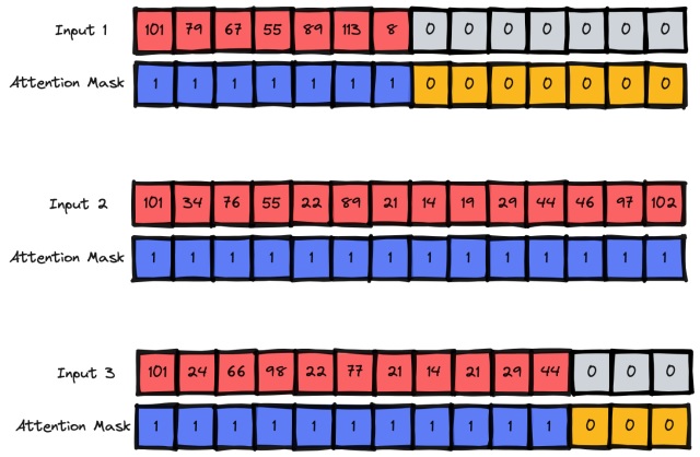
{'input_ids': [[101, 1045, 2134, 2102, 2514, 26608, 102, 0, 0, 0, 0, 0, 0, 0, 0, 0, 0, 0, 0, 0, 0, 0, 0], [101, 1045, 2064, 2175, 2013, 3110, 2061, 20625, 2000, 2061, 9636, 17772, 2074, 2013, 2108, 2105, 2619, 2040, 14977, 1998, 2003, 8300, 102], [101, 10047, 9775, 1037, 3371, 2000, 2695, 1045, 2514, 20505, 3308, 102, 0, 0, 0, 0, 0, 0, 0, 0, 0, 0, 0]], 'attention_mask': [[1, 1, 1, 1, 1, 1, 1, 0, 0, 0, 0, 0, 0, 0, 0, 0, 0, 0, 0, 0, 0, 0, 0], [1, 1, 1, 1, 1, 1, 1, 1, 1, 1, 1, 1, 1, 1, 1, 1, 1, 1, 1, 1, 1, 1, 1], [1, 1, 1, 1, 1, 1, 1, 1, 1, 1, 1, 1, 0, 0, 0, 0, 0, 0, 0, 0, 0, 0, 0]]}

We get a larger amount of the same type of output but this lets me show a few things. First, consider the “input_ids” in sequence to make it easier:

[101, 1045, 2134, 2102, 2514, 26608, 102, 0, 0, 0, 0, 0, 0, 0, 0, 0, 0, 0, 0, 0, 0, 0, 0]

[101, 1045, 2064, 2175, 2013, 3110, 2061, 20625, 2000, 2061, 9636, 17772, 2074, 2013, 2108, 2105, 2619, 2040, 14977, 1998, 2003, 8300, 102]

[101, 10047, 9775, 1037, 3371, 2000, 2695, 1045, 2514, 20505, 3308, 102, 0, 0, 0, 0, 0, 0, 0, 0, 0, 0, 0]

Notice those zeros in the input_ids for two of the entries. Here zeros have been added to make everything the same length. These zeros will correspond to a [PAD] token that gets placed into the vocabulary.

In fact, as part of our diagnostic print statements, you should see the following:

['[CLS]', 'i', 'didn', '##t', 'feel', 'humiliated', '[SEP]', '[PAD]', '[PAD]', '[PAD]', '[PAD]', '[PAD]', '[PAD]', '[PAD]', '[PAD]', '[PAD]', '[PAD]', '[PAD]', '[PAD]', '[PAD]', '[PAD]', '[PAD]', '[PAD]']

The [PAD] tokens are what they sound like: padding. Padding is added to make sure all sequences in a batch have the same length, which is necessary for processing by most models. In this case, the sequence is padded with a number of [PAD] tokens to match the length of the longest sequence in the batch.

With this output, also notice those attention_mask elements. Again, in sequence, to make them a bit easier to reason about:

[1, 1, 1, 1, 1, 1, 1, 0, 0, 0, 0, 0, 0, 0, 0, 0, 0, 0, 0, 0, 0, 0, 0]

[1, 1, 1, 1, 1, 1, 1, 1, 1, 1, 1, 1, 1, 1, 1, 1, 1, 1, 1, 1, 1, 1, 1]

[1, 1, 1, 1, 1, 1, 1, 1, 1, 1, 1, 1, 0, 0, 0, 0, 0, 0, 0, 0, 0, 0, 0]

We now have a bunch of zeroes in that list as well and this is because the model shouldn’t be using the additional padding tokens for any sort of learning. Thus the attention mask lets the model ignore the padded parts of the input.

You can now extrapolate this to all of the data in the dataset. All input sequences of text will be padded to the maximum sequence length in a given batch. The attention masks applied to the data, and used in the model, will be set to ignore any padded areas of the data.

What I hope this shows you is that you can be aware of what data you are pulling in and how a pre-trained model is tokenizing it and encoding it.

In previous posts, we had mostly built our own simple tokenizers and encoders so we knew exactly what was going on. Here I’m just making sure that when you use existing work by others, it doesn’t have to be a black box to you.

Modularize Your Script

Before moving on, let’s do something I talked about at the end of the last post. Let’s create a function for what we just did so that we can more easily call it on any batched amount of data. Here’s a modified version of the script.

You’ll get the same output as before. Beyond modularizing our code for clarity, there actually is another reason for doing this.

Mapping Our Actions to Data

We’re obviously passing in batches to our function, which was the purpose of using our datum variable and changing the range from [:1] to [:3]. But clearly that’s more for illustrative purposes. So let’s remove our datum variable. Instead put this in place:

When running this code, you’ll see that a map operation is occurring:

Map: 16000/16000
Map: 2000/2000
Map: 2000/2000

But what’s actually happening here? Well, first let’s notice the output you get:

DatasetDict({
  train: Dataset({
    features: ['text', 'label', 'input_ids', 'attention_mask'],
    num_rows: 16000
  })
  validation: Dataset({
    features: ['text', 'label', 'input_ids', 'attention_mask'],
    num_rows: 2000
  })
  test: Dataset({
    features: ['text', 'label', 'input_ids', 'attention_mask'],
    num_rows: 2000
  })
})

Notice the “features” here have been added to. And we can verify that by checking our column names, like we did earlier in this post.

This is crucial! We have added these elements to our features. And remember that features are what the learning model considers as it trains.

But let’s go back to that operation. What are we doing with the code we added?

The map() method is a convenient way to apply a function to each item in a dataset. Once we’ve defined a processing function, like the tokenize one we defined, that function can be applied across all the splits in the dataset in just a single line of code.

By default, the map() method operates individually on every example in the dataset.

Setting “batched=True”, as we did, will encode the text in batches. This parameter indicates that the function should be applied in batches rather than element-wise. This is actually fairly important so let’s clarify this terminology.

When processing data “in batches,” you group multiple data points (or elements) together and apply an operation to the entire group simultaneously. This is useful for operations that can be parallelized. This is because it allows for more efficient processing on modern hardware. For example, if you have a dataset of sentences and you want to tokenize them using a tokenizer, processing several sentences at once in a batch can be faster than processing each sentence individually.

When processing data “element-wise,” you apply an operation to each individual data point separately. This is the traditional way of processing data, where you iterate through each element and perform the operation on it. It’s useful for operations that need to consider each element independently, without interaction or grouping.

As you might guess, using the batches approach can significantly speed up the processing, as many operations can be parallelized across the batch.

Because we’ve set “batch_size=None”, our tokenize() function will be applied on the full dataset as a single batch. One thing this does for us is allow our logic to take advantage of maximum parallelization.

However, this also ensures that the input tensors and attention masks have the same shape across the entire dataset. This is because all the samples are being processed together as one batch, so their shapes align. That “shape” is determined by the maximum sequence length in the batch, hence that need for padding that we looked at earlier.

Feed the Model

Let’s take a moment to consider what we’re going to be feeding our data into. What we’re using is an encoder-based model. Specifically we’re passing in a sequence of encoded tokens. Thus while we call our work text classification, what we’re really doing is sequence classification.

Encoder-based models have an architecture that’s well-suited to handle this sequence-based work. This architecture has two main components we can consider: a pre-trained body and a custom classification head.

What does all that mean?

A “pretrained body” refers to the encoder part of that model that has been pre-trained on a large dataset (or “corpus”) of text data. This pre-training step helps the model learn rich representations of language and captures various linguistic features. This is what DistilBERT basically is.

The “classification head” refers to the part of the model that’s added on top of the pre-trained encoder to adapt it to the specific classification task at hand. This head typically consists of one or more layers that take the high-level encoded representations from the encoder and transform them into the appropriate format for the classification task. For sequence classification tasks, this can involve various different things.

Some of those “different things” are adding what’s called a softmax layer for multi-class classification or adding what’s called a sigmoid layer for binary classification.

Here’s a rough idea of what this architecture looks like.

Let’s consider what’s going on there.

First, the input text undergoes tokenization. By now, you certainly know this involves a process of segmenting the text into smaller linguistic units known as tokens. These tokens are then encoded into one-hot vectors, resulting in token encodings. The dimensionality of these encodings is determined by the vocabulary size of the tokenizer.

Next, these token encodings are transformed into token embeddings. These are lower-dimensional continuous vectors. These embeddings capture the semantic relationships between tokens and allow for more efficient processing compared to the initial higher-dimensional one-hot representations.

Encoding vs Embedding

The distinction I just brought up can actually be a little confusing. At least it was to me. So let’s go back to one of our examples:

Text: 'i didnt feel humiliated'
Encoding: [1045, 2134, 2102, 2514, 26608]

We know that text gets tokenized and special tokens are included, so we end up with:

Tokenized: ['i', 'didn', 't', 'feel', 'humiliated']
Encoded: [101, 1045, 2134, 2102, 2514, 26608, 102]

All those token numerical IDs are then used to look up the corresponding token embeddings from what’s called the embedding matrix of the pre-trained model. Each token ID corresponds to a vector in the embedding space. These vectors represent the semantic features of the individual tokens.

The term “embedding matrix” refers to a two-dimensional array that stores the vector representations of tokens, words, or other discrete elements in a lower-dimensional space. The token IDs we have from our endoding correspond to rows in the embedding matrix of a pre-trained model like DistilBERT.

Here’s a hypothetical embedding matrix for this small vocabulary:

Token        |  Dimension 1  |  Dimension 2
-------------------------------------------
"i"          |     0.2       |     0.5
"didnt"      |    -0.3       |     0.1
"feel"       |     0.7       |    -0.2
"humiliated" |     0.9       |     0.6

In this example, the embedding matrix is a 4×2 matrix, where each row corresponds to a token, and each column corresponds to a dimension in the embedding space. The values in the matrix represent the embedding values for each token along each dimension.

When you want to access the embedding for a specific token — say, “feel” — you look up its corresponding row in the matrix. For example, the embedding for “feel” would be [0.7, -0.2].

Again, please note that in real-world scenarios, embedding matrices are much larger — often hundreds or thousands of dimensions — and represent a more complex semantic space.

Our simple example illustrates the basic idea of how tokens are mapped to embeddings in an embedding matrix.

But you might ask: why does “feel” exist in two dimensions? Put another way: why is there a dimension 1 and dimension 2 for each token?

The reason tokens like “feel” exist in two dimensions — or more — in the embedding matrix is because each dimension captures a different aspect of the token’s meaning or relationship to other tokens. Put another way, each dimension in the embedding space represents a feature or characteristic of the token.

Let’s dive deeper into this concept, because this is where the distinction between encodings and embeddings really comes in.

The multidimensional representation is necessary because words or tokens can have complex relationships and meanings that can’t be fully captured in a single dimension. By using multiple dimensions, we can represent different aspects of a token’s semantic information. Each dimension can be thought of as capturing a different linguistic feature, like sentiment, tense, gender, etc.

We also have to consider semantic similarity. Tokens with similar meanings or contextual usage tend to have similar embeddings. For example, words that are synonyms or have similar semantic relationships might have embeddings that are closer to each other in the embedding space.

There’s also the idea of analogies and relationships. The embedding space allows for algebraic operations like word analogies. For example, "king" - "man" + "woman" might yield an embedding that’s close to "queen". These operations work because different dimensions contribute to capturing the relationships between words.

Crucially, in the context of neural networks, and thus learning models, the model learns to adjust the values in the embedding matrix during training to optimize performance on the specific task. The dimensions allow the model to capture different levels of abstraction and relationships in the data.

It’s pretty powerful stuff and I’m only scratching the surface here.

Back To Our Architecture

The token embeddings we just talked about are fed through a series of encoder block layers, each incorporating attention mechanisms and feedforward neural networks. These encoder blocks analyze the tokens in context, producing a hidden state for each token.

“Encoder block layers” refer to a critical component within the architecture of many neural network models designed for natural language processing tasks. These layers play a key role in capturing the contextual information and relationships between tokens in a sequence of text.

Let’s talk about those hidden states for a second because they do relate to the embedding matrix we just talked about.

The hidden state contains contextual information derived from the surrounding tokens. The hidden states can be thought of as contextually enriched representations of tokens. Or, put another way, the hidden states can be thought of as dynamic and contextualized versions of the token embeddings.

The hidden states contain information about how each token relates to its surrounding tokens in the specific context of the sequence being processed. So, while the initial embeddings come from the embedding matrix lookups, the hidden states are the result of processing these embeddings through the encoder block layers, capturing higher-level contextual information.

It’s actually really hard to visualize this given the dimensions of text representations. But consider this idea of image classification:

Here the “visible layer” would correspond to our text. The “output” would correspond to our classification. Those hidden layers are very similar, at least conceptually, to the hidden states I’m talking about.

The commonality here is learned representations. In both text and image processing, these learned representations enable models to extract meaningful and relevant features from the input data, enhancing their ability to perform classification tasks effectively.

During the pre-training phase, which is often accomplished through language modeling, each hidden state serves a dual purpose. The first purpose is what I described above: contextual relationships. The other is that the hidden state is utilized to predict masked input tokens, contributing to the model’s understanding of those contextual relationships. This pre-training phase helps the model capture the underlying patterns of the language.

“Masked input tokens” refer to a specific training technique used in language modeling tasks, where certain tokens in the input text are intentionally replaced or “masked” during training. This technique encourages the model to predict the original tokens based on their surrounding context.

All this being said However, for a classification task, the architecture diverges a bit.

The pre-training-focused language modeling layer is substituted with a classification layer.

This dedicated layer takes the contextual hidden states from the encoder blocks and transforms them into predictions specific to the classification classes. This adaptation enables the model to repurpose its learned language understanding for accurate classification.

And that’s what we’re aiming to do: classify.

There are two distinct approaches for training a model on our dataset using a pre-trained language model, which is what our DistilBERT model is. So let’s talk about that a bit.

The Basis of Training

One of the core approaches here is called feature extraction.

In the previous post, we talked a lot about hidden states. With a feature extraction approach, you use the hidden states produced by the pre-trained language model as features for your classification task.

Remember that these hidden states contain rich contextual information about the input text. You don’t modify the parameters of the pre-trained model; instead, you attach a separate classifier on top of these hidden states. This classifier is then trained specifically for the classification task you care about, which in our case is sentiment analysis.

There is another approach that’s common here which is called fine-tuning. This approach expands on what I just talked about. Not only do you use the hidden states for your classification task, but you also allow the parameters of the pre-trained model — both the encoder and the classification head — to be updated during training. This means that the model can adapt its learned representations to the specifics of your dataset and task.

In the above visual, the orange blocks, with the arrows underneath them, represent the updating of the parameters.

Both approaches have their merits and trade-offs. Feature extraction is often faster and requires less computational power, while fine-tuning allows the model to adapt to the dataset more closely but is more computationally intensive.

In fact, fine-tuning requires a lot more computation in some cases, which can mean you must have GPUs available to do the processing. Since I can’t guarantee everyone’s setup and since I’m not showing these examples in a cloud-based infrastructure, I’m only going to focus on the feature extraction part here.

Extracting Features

In this approach, you’re using a pre-trained language model’s capabilities to extract valuable features (hidden states) from the input text data. These features will then be used as input to a separate classifier to perform the specific sentiment analysis task.

Here we freeze the encoder layer during training. Or, put more accurately, we freeze the weights that the encoder layer uses during training.

Keep in mind these layers are responsible for processing the input text. “Freezing the weights” means that you prevent these encoder layers from being updated or modified during the training of the classifier. This ensures that the learned representations — again, the hidden states — extracted from the pre-trained model are retained and not altered during the subsequent training.

So Let’s remind ourselves of our architecture that we looked at earlier.

So here’s a breakdown of the concepts I’ve just talked about:

• As the input text passes through the pre-trained language model’s encoder layers, it generates hidden states at various levels of abstraction.
• These hidden states capture contextual information about the text.
• In the feature extraction approach, these hidden states are treated as features for the classifier.
• Each hidden state can be considered a feature vector that encodes information about the input text’s content and context.

This feels like a good breaking point and so in the next, and final, post in this series we’ll actually train our model on our dataset and see what results we actually get.